Growing tube model

In this tutorial, you will use the growing tube model (Okamoto, 1988) in both directions: generate shells from parameters, including heteromorph (irregularly coiled) shells, and estimate the parameters from a shell.

The growing tube model describes a coiling pattern using a differential-geometric framework. The tube radius and the trajectory’s local geometry are set by three parameters at each growth stage s:

• expansion rate e_g: how fast the tube radius grows

• standardized curvature c_g: how tightly the trajectory bends (c_g = 0 is a straight tube)

• standardized torsion t_g: how much the trajectory twists out of a plane (t_g = 0 is a planispiral)

Setup

# Uncomment if needed
# %pip install "ktch[plot]"

import matplotlib.pyplot as plt
import numpy as np
import pandas as pd
import plotly.graph_objects as go
from plotly.subplots import make_subplots

from ktch.coiling import GrowingTubeModel, growing_tube
from ktch.plot import morphospace_plot

Show definitions: plot_surface3d(), plot_surface_grid()

Hide definitions: plot_surface3d(), plot_surface_grid()

def plot_surface3d(X, *, title="", colorscale="Viridis"):
    """Plot a ``(n, n_phi, 3)`` surface array with plotly."""
    x, y, z = X[..., 0], X[..., 1], X[..., 2]
    fig = go.Figure(
        data=[go.Surface(x=x, y=y, z=z, colorscale=colorscale, showscale=False)]
    )
    fig.update_layout(
        title=title,
        width=700,
        height=500,
        scene=dict(aspectmode="data"),
    )
    return fig


def plot_surface_grid(surfaces, subplot_titles, *, ncols=None, title="",
                      colorscale="Viridis"):
    """Lay out ``(n_s, n_phi, 3)`` surface arrays in a grid of subplots."""
    n = len(surfaces)
    ncols = n if ncols is None else ncols
    nrows = int(np.ceil(n / ncols))
    fig = make_subplots(
        rows=nrows,
        cols=ncols,
        specs=[[{"type": "surface"}] * ncols] * nrows,
        subplot_titles=list(subplot_titles),
        horizontal_spacing=0.01,
        vertical_spacing=0.05,
    )
    scenes = {}
    for i, Xi in enumerate(surfaces):
        row, col = divmod(i, ncols)
        fig.add_trace(
            go.Surface(
                x=Xi[..., 0],
                y=Xi[..., 1],
                z=Xi[..., 2],
                showscale=False,
                colorscale=colorscale,
            ),
            row=row + 1,
            col=col + 1,
        )
        scenes["scene" if i == 0 else f"scene{i + 1}"] = dict(aspectmode="data")
    fig.update_layout(
        title=title,
        width=900,
        height=350 * nrows,
        margin=dict(l=0, r=0, t=60, b=0),
        **scenes,
    )
    return fig

Generate your first shell

GrowingTubeModel provides the model. Its inverse_transform takes the parameters and returns a sampled surface. We also pass a sampling grid (s_range along the growth trajectory, phi_range around the aperture).

The method argument of the model selects the solver. With constant parameters, the closed form (method="closed") is exact and fast; the default method="ode" integrates the growth equations and is required for non-constant parameters (see the heteromorph section below).

s = np.linspace(0.0, 60.0, 200)
phi = np.linspace(0.0, 2.0 * np.pi, 60)

growing_tube_model = GrowingTubeModel(method="closed")
X = growing_tube_model.inverse_transform([0.02, 0.4, 0.06], s_range=s, phi_range=phi)
X.shape

(200, 60, 3)

The result is a (n_s, n_phi, 3) array: n_s samples along the growth stage s, n_phi samples around the tube, and the (x, y, z) coordinates.

fig = plot_surface3d(X, title="Growing tube (e_g=0.02, c_g=0.4, t_g=0.06)")
fig.show()

Orientation of the aperture

The full parameter vector of GrowingTubeModel has five entries:

growing_tube_model.get_feature_names_out()

array(['e_g', 'c_g', 't_g', 'delta_g', 'gamma_g'], dtype='<U7')

The last two, delta_g and gamma_g, set the orientation of the aperture within the moving (Frenet) frame of the trajectory; (0, 0) keeps the aperture perpendicular to the growth direction. A 3-entry input, as above, sets both to zero.

Passing a (n_samples, 5) array to inverse_transform generates one surface per row, so a comparison is a single call:

params = np.array(
    [
        [0.02, 0.4, 0.06, 0.0, 0.0],
        [0.02, 0.4, 0.06, 0.4, 0.0],
        [0.02, 0.4, 0.06, 0.0, 0.4],
    ]
)
surfaces = growing_tube_model.inverse_transform(params, s_range=s, phi_range=phi)
surfaces.shape

(3, 200, 60, 3)

plot_surface_grid(
    surfaces,
    ["delta_g=0, gamma_g=0", "delta_g=0.4, gamma_g=0", "delta_g=0, gamma_g=0.4"],
    title="Orientation of the aperture",
).show()

The leading axis indexes the parameter rows; the rest is the familiar (n_s, n_phi, 3) surface.

Explore the parameters

We vary one parameter while holding the other two constant to see each effect. All sweeps share the growth span s. One revolution of the trajectory advances s by 2 * pi / hypot(c_g, t_g), so a tighter coil shows more whorls over the same span.

Expansion rate e_g

With e_g = 0 the tube keeps a constant radius; larger values expand the aperture quickly.

params = np.array([[0.0, 0.4, 0.06], [0.04, 0.4, 0.06], [0.2, 0.4, 0.06]])
plot_surface_grid(
    growing_tube_model.inverse_transform(params, s_range=s, phi_range=phi),
    ["e_g=0.0", "e_g=0.04", "e_g=0.2"],
    title="Expansion rate",
).show()

Standardized curvature c_g

Larger values give a tighter coil. (At c_g = 0 the trajectory becomes straight.)

params = np.array([[0.04, 0.0, 0.06], [0.04, 0.4, 0.06], [0.04, 0.8, 0.06]])
plot_surface_grid(
    growing_tube_model.inverse_transform(params, s_range=s, phi_range=phi),
    ["c_g=0.0", "c_g=0.4", "c_g=0.8"],
    title="Standardized curvature",
).show()

Standardized torsion t_g

With t_g = 0 the coil stays planar (a planispiral); increasing it lifts it into a helix.

params = np.array([[0.04, 0.4, 0.0], [0.04, 0.4, 0.06], [0.04, 0.4, 0.2]])
plot_surface_grid(
    growing_tube_model.inverse_transform(params, s_range=s, phi_range=phi),
    ["t_g=0.0", "t_g=0.06", "t_g=0.2"],
    title="Standardized torsion",
).show()

Heteromorph

So far the parameters were constant, giving regular spirals. The growing tube model naturally allows its parameters (e_g, c_g, and t_g) to change during growth. The function growing_tube() accepts each of them as a function of the growth stage s (or an array aligned to s_range). This produces heteromorph (irregularly coiled) shells.

The example below mimics the heteromorph ammonite Nipponites (Okamoto, 1988): a constant expansion rate with curvature and torsion that oscillate along growth.

e_g = np.log(1.028)

def c_g(s):
    return 0.2 * np.sin(2.0 * np.pi * s / 7.0 - np.pi / 2.0) + 0.5

def t_g(s):
    return 0.55 * np.cos(2.0 * np.pi * s / 14.0)

Let’s look at the two varying parameters as functions of s:

s_het = np.linspace(0.0, 45.0, 451)

fig = go.Figure()
fig.add_scatter(x=s_het, y=c_g(s_het), mode="lines", name="c_g(s)")
fig.add_scatter(x=s_het, y=t_g(s_het), mode="lines", name="t_g(s)")
fig.update_layout(width=700, height=300, xaxis_title="s", yaxis_title="value")
fig.show()

Non-constant parameters require method="ode" (the closed form only handles constant parameters) and an explicit s_range.

X_het = growing_tube(e_g, c_g, t_g, s_range=s_het, method="ode",
                     phi_range=np.linspace(0.0, 2.0 * np.pi, 40))
plot_surface3d(X_het, title="Nipponites-like heteromorph", colorscale="Purp").show()

Try changing the oscillation periods (7 and 14) or amplitudes to explore other irregular forms.

Note

GrowingTubeModel currently works with constant parameters: inverse_transform takes rows of numbers, and transform (next section) estimates a single parameter vector per shell. Heteromorph shells are generated with growing_tube(); estimating their varying parameters is not supported yet and is planned for a future release.

Estimate the parameters

Now, the reverse direction. transform takes a shell surface and estimates the parameters from it. The "surface" method fits the model directly to a structured surface.

Note

The default estimator="nls_3d" expects a sequence of centroid and thickness measurements (x, y, z, r) along a specimen and is not covered here.

We generate a shell with a known parameter vector, including the orientation, and then try to estimate it.

s = np.linspace(0.0, 50.0, 180)

params_true = np.array([0.05, 0.24, 0.05, 0.3, -0.2])
X = growing_tube_model.inverse_transform(params_true, s_range=s, phi_range=phi)

growing_tube_model.set_params(estimator="surface")
params_est = growing_tube_model.transform(X)
params_est.shape

(1, 5)

set_params selects the estimation method; inverse_transform is not affected. transform works on a panel of surfaces. The result has one row per surface. A single (n_s, n_phi, 3) array is accepted as a panel of one.

pd.DataFrame(
    {"true": params_true, "estimated": params_est[0]},
    index=growing_tube_model.get_feature_names_out(),
)

	true	estimated
e_g	0.05	0.05
c_g	0.24	0.24
t_g	0.05	0.05
delta_g	0.30	0.30
gamma_g	-0.20	-0.20

You should see the five parameters recovered to numerical precision. The "surface" method fits the rigid pose and the initial radius of the surface together with the parameters. It does not require the shell to sit in any particular position, orientation, or scale.

To close the loop, generate a shell from the estimate and compare it with the original:

X_rec = growing_tube_model.inverse_transform(params_est[0], s_range=s, phi_range=phi)

rmsd = np.sqrt(np.mean(np.sum((X_rec - X) ** 2, axis=-1)))
print(f"root-mean-square distance: {rmsd:.2e}")

root-mean-square distance: 2.08e-14

fig = go.Figure(
    data=[
        go.Surface(
            x=X[..., 0], y=X[..., 1], z=X[..., 2],
            colorscale="Viridis", opacity=0.8, showscale=False,
        ),
        go.Surface(
            x=X_rec[..., 0], y=X_rec[..., 1], z=X_rec[..., 2],
            colorscale="Reds", opacity=0.4, showscale=False,
        ),
    ]
)
fig.update_layout(
    title="Original (Viridis) and reconstruction (Reds)",
    width=700,
    height=500,
    scene=dict(aspectmode="data"),
)
fig.show()

The two surfaces coincide. This is the sense in which transform and inverse_transform are inverses of each other: a parameter vector, the shell it generates, and the parameters estimated from that shell describe the same form.

Note

The "surface" method assumes that rows run along the growth stage and columns run once around the tube, as in the output of inverse_transform. It uses the coordinates only: the grid values s_range and phi_range are not needed. A surface generated with method="ode" is estimated the same way.

Many shells at once

Both directions work on batches. A (n_samples, 5) parameter array gives a (n_samples, n_s, n_phi, 3) panel, and transform on that panel gives the parameters back row by row.

params_batch = np.array(
    [
        [0.05, 0.24, 0.05, 0.0, 0.0],
        [0.03, 0.20, 0.00, 0.1, 0.1],
        [0.10, 0.40, 0.15, -0.2, 0.2],
    ]
)
surfaces = growing_tube_model.inverse_transform(params_batch, s_range=s, phi_range=phi)
estimates = growing_tube_model.transform(surfaces)

pd.DataFrame(estimates, columns=growing_tube_model.get_feature_names_out())

	e_g	c_g	t_g	delta_g	gamma_g
0	0.05	0.24	5.000000e-02	-5.272290e-17	-5.477210e-17
1	0.03	0.20	4.266952e-20	1.000000e-01	1.000000e-01
2	0.10	0.40	1.500000e-01	-2.000000e-01	2.000000e-01

print(f"largest absolute error: {np.max(np.abs(estimates - params_batch)):.2e}")

largest absolute error: 1.75e-15

For analysis pipelines, pass as_frame=True to get a tidy long-format DataFrame indexed by (specimen_id, trajectory_id, phi_id). transform accepts this frame as well.

df = growing_tube_model.inverse_transform(
    params_batch, s_range=s, phi_range=phi, as_frame=True
)
df.head()

			x	y	z
specimen_id	trajectory_id	phi_id
0	0	0	0.0	1.000000	0.000000
		1	0.0	0.994335	0.106293
		2	0.0	0.977403	0.211383
		3	0.0	0.949398	0.314077
		4	0.0	0.910635	0.413212

Morphospace

A theoretical morphospace is the parameter space viewed through the shells it generates. morphospace_plot from ktch.plot draws a scatter plot in a two-dimensional space and places generated shapes at a regular grid of positions. It expects a reducer (such as PCA) between the axes and the descriptor; here the axes are the parameters c_g and t_g themselves, so the reducer is the identity, and the descriptor is inverse_transform with e_g fixed.

e_fixed = 0.04


def shells_at(c_t):
    """Generate one four-whorl shell per ``(c_g, t_g)`` row at ``e_g = e_fixed``."""
    return np.stack(
        [
            growing_tube_model.inverse_transform(
                [e_fixed, c, t],
                s_range=np.linspace(0.0, 2.0 * np.pi * 4.0 / np.hypot(c, t), 120),
                phi_range=np.linspace(0.0, 2.0 * np.pi, 30),
            )
            for c, t in np.asarray(c_t)
        ]
    )


fig, ax = plt.subplots(figsize=(7, 6))
ax.set_xlim(0.1, 0.9)
ax.set_ylim(-0.05, 0.25)
morphospace_plot(
    reducer_inverse_transform=lambda scores: scores,  # axes are the parameters
    n_components=2,
    descriptor_inverse_transform=shells_at,
    n_shapes=3,
    shape_scale=0.9,
    ax=ax,
)
ax.scatter(estimates[:, 1], estimates[:, 2], zorder=2)
for i, (c, t) in enumerate(estimates[:, 1:3]):
    ax.annotate(f"shell {i}", (c, t), xytext=(5, 5), textcoords="offset points")
ax.set_xlabel("c_g (standardized curvature)")
ax.set_ylabel("t_g (standardized torsion)")
ax.set_title("Morphospace over c_g and t_g (e_g=0.04)");

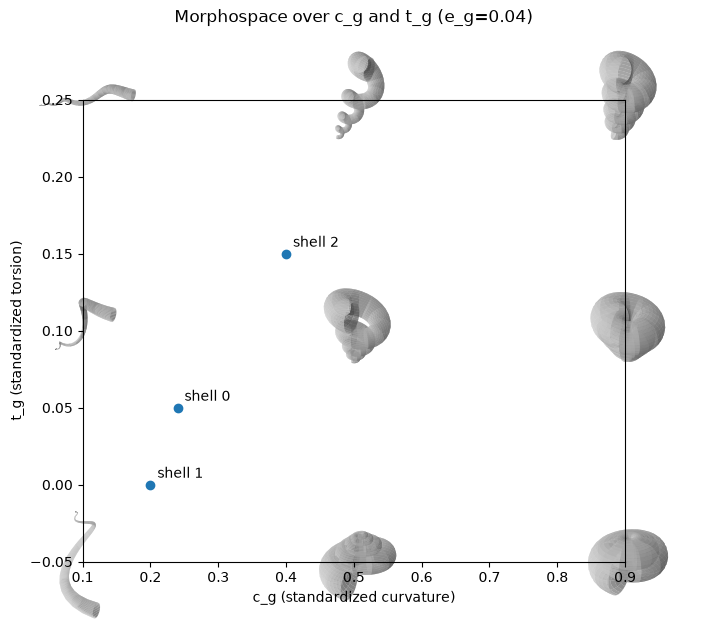
The insets show the shells generated at the grid positions; the points are the shells estimated in the previous section. Generation places a shell at a point of the morphospace; estimation reads the point back from the shell. Use the first to design shells and the second to locate specimens.

See also

• Raup’s model to do the same with Raup’s model.

• Sample evenly along a coiled shell to space the samples evenly along the shell instead of evenly in s.

• Theoretical morphological models of coiling for the theory behind the growing tube model, including the differential geometry of heteromorph growth.

References

• Okamoto, T., 1988. Analysis of heteromorph ammonoids by differential geometry. Palaeontology 31, 35–52.