Use Non-PCA Reducers#
Use KernelPCA or other reducers with ktch plot functions via explicit override parameters.
The reducer convenience parameter targets PCA-compatible estimators.
For reducers with different attribute names (e.g., KernelPCA stores
eigenvalues in eigenvalues_ instead of explained_variance_), pass
the override parameters directly:
reducer_inverse_transform: callable that maps scores back to coefficient spacen_components: total number of componentscomponent_std: per-component standard deviation for SD scaling (shape_variation_plotonly)descriptor_inverse_transform: callable that maps coefficients to shape coordinates (optional; can also usedescriptor)
Setup#
import numpy as np
import pandas as pd
import matplotlib.pyplot as plt
from sklearn.decomposition import KernelPCA

from ktch.datasets import load_outline_mosquito_wings
from ktch.harmonic import EllipticFourierAnalysis
from ktch.plot import shape_variation_plot, morphospace_plot

data = load_outline_mosquito_wings(as_frame=True)
coords = data.coords.to_numpy().reshape(-1, 100, 2)

efa = EllipticFourierAnalysis(n_harmonics=20)
coef = efa.fit_transform(coords)

kpca = KernelPCA(n_components=5, kernel="rbf", fit_inverse_transform=True)
kpca.fit(coef)
KernelPCA(fit_inverse_transform=True, kernel='rbf', n_components=5)In a Jupyter environment, please rerun this cell to show the HTML representation or trust the notebook.
On GitHub, the HTML representation is unable to render, please try loading this page with nbviewer.org.
Parameters
Fitted attributes
5 features
| kernelpca0 |
| kernelpca1 |
| kernelpca2 |
| kernelpca3 |
| kernelpca4 |
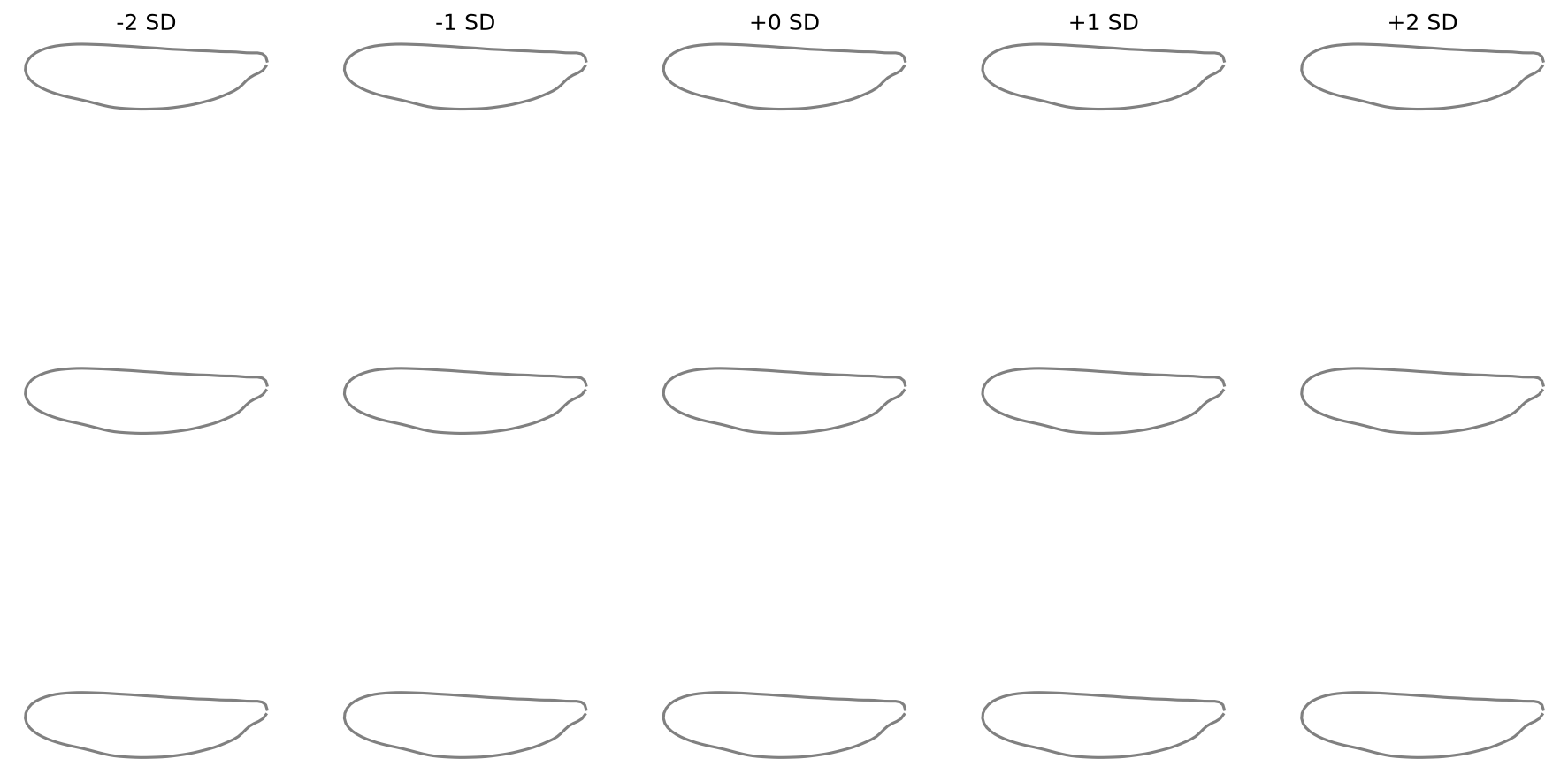
Shape variation with KernelPCA#
Compute the per-component standard deviation from the actual scores
and pass it via component_std. This works for any reducer:
scores = kpca.transform(coef)

fig = shape_variation_plot(
    reducer_inverse_transform=kpca.inverse_transform,
    component_std=np.std(scores, axis=0),
    n_components=kpca.n_components,
    descriptor=efa,
    components=(0, 1, 2),
)
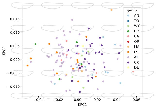
Morphospace with KernelPCA#
scores = kpca.transform(coef)
df_kpca = pd.DataFrame(
    scores[:, :2], columns=["KPC1", "KPC2"],
)
df_kpca.index = data.meta.index
df_kpca = df_kpca.join(data.meta)

ax = morphospace_plot(
    data=df_kpca,
    x="KPC1", y="KPC2", hue="genus",
    reducer_inverse_transform=kpca.inverse_transform,
    n_components=kpca.n_components,
    descriptor=efa,
    palette="Paired",
    n_shapes=5,
)
See also
Visualize Morphospace for standard PCA morphospace visualization
Visualize Shape Variation for shape variation along component axes
Morphometric Visualization for the convenience vs override parameter design