2D Outline Registration#
Align 2D outlines by adjusting position, orientation, scale, and starting point before EFA.
import numpy as np
import scipy as sp

import matplotlib.pyplot as plt
import seaborn as sns

from ktch.datasets import load_outline_mosquito_wings
data_outline_mosquito_wings = load_outline_mosquito_wings(as_frame=True)
coords = data_outline_mosquito_wings.coords.to_numpy().reshape(-1,100,2)
Translation#
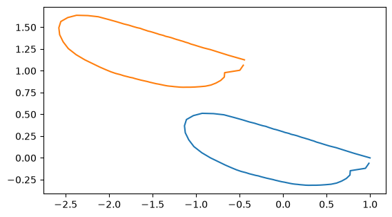
You can translate the coordinate values of outline data using list comprehension.
rng = np.random.default_rng()
dx = rng.normal(0, 1, size=coords.shape[0::2])
coords_translated = [coords[i] + dx[i] for i in range(len(coords))]
idx = 0

fig, ax = plt.subplots()
sns.lineplot(x=coords[idx][:,0], y=coords[idx][:,1], sort= False,estimator=None,ax=ax)
sns.lineplot(x=coords_translated[idx][:,0], y=coords_translated[idx][:,1], sort= False,estimator=None,ax=ax)
ax.set_aspect('equal')
print("displacement: ", dx[idx])
displacement: [-1.44464982 1.12580515]
If the coordinate values are stored as np.ndarray,
you can simply add the displacement vectors after reshape(n_specimens, 1, n_dim).
coords_translated_array = coords + dx.reshape(dx.shape[0], 1, dx.shape[1])

idx = 0

fig, ax = plt.subplots()
sns.lineplot(x=coords[idx][:,0], y=coords[idx][:,1], sort= False,estimator=None,ax=ax)
sns.lineplot(x=coords_translated_array[idx][:,0], y=coords_translated_array[idx][:,1], sort= False,estimator=None,ax=ax)
ax.set_aspect('equal')
print("displacement: ", dx[idx])
displacement: [-1.44464982 1.12580515]
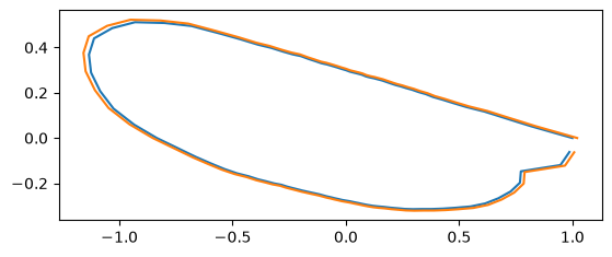
Scaling#
s = rng.uniform(0.5,1.5, size=coords.shape[0])
coords_scaled = [s[i]*coords[i] for i in range(len(coords))]
idx = 0

fig, ax = plt.subplots()
sns.lineplot(x=coords[idx][:,0], y=coords[idx][:,1], sort= False,estimator=None,ax=ax)
sns.lineplot(x=coords_scaled[idx][:,0], y=coords_scaled[idx][:,1], sort= False,estimator=None,ax=ax)
ax.set_aspect('equal')
print("scale: ", s[idx])
scale: 1.0212535628490813
If the coordinate values are stored as np.ndarray,
you can simply add the displacement vectors after reshape(n_specimens, 1, 1).
coords_scaled_arr = s.reshape(s.shape[0], 1, 1)*coords

idx = 0

fig, ax = plt.subplots()
sns.lineplot(x=coords[idx][:,0], y=coords[idx][:,1], sort= False,estimator=None,ax=ax)
sns.lineplot(x=coords_scaled_arr[idx][:,0], y=coords_scaled_arr[idx][:,1], sort= False,estimator=None,ax=ax)
ax.set_aspect('equal')
print("scale: ", s[idx])
scale: 1.0212535628490813
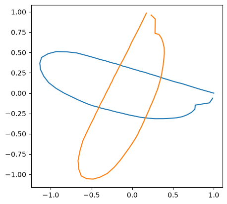
Rotation#
We provide rotation_matrix_2d helper function to generate the rotation matrix.
Alternatively, you can use scipy.spatial.transform.Rotation or define by yourself.
from ktch.harmonic import rotation_matrix_2d
from scipy.spatial.transform import Rotation as R
theta = np.pi/4
print(rotation_matrix_2d(theta))
print(R.from_rotvec(theta*np.array([0,0,1])).as_matrix()[0:2,0:2])
print(np.array([[np.cos(theta),-np.sin(theta)],[np.sin(theta), np.cos(theta)]]))
[[ 0.70710678 -0.70710678]
 [ 0.70710678  0.70710678]]
[[ 0.70710678 -0.70710678]
 [ 0.70710678  0.70710678]]
[[ 0.70710678 -0.70710678]
 [ 0.70710678  0.70710678]]
theta = rng.uniform(0, 2*np.pi, size=coords.shape[0])
coords_rotated = [(rotation_matrix_2d(theta[i]) @ coords[i].T).T for i in range(len(coords))]
idx = 0

fig, ax = plt.subplots()
sns.lineplot(x=coords[idx][:,0], y=coords[idx][:,1], sort= False,estimator=None,ax=ax)
sns.lineplot(x=coords_rotated[idx][:,0], y=coords_rotated[idx][:,1], sort= False,estimator=None,ax=ax)
ax.set_aspect('equal')
print("theta: ", theta[idx])
theta: 1.3969513254185506
When the coordinate values are stored as np.ndarray,
the rotated array is calculated by applying the matmul (@) operator on the array of rotation matrixes transposed to n_samples x n_dim x n_dim and the array of the coordinate values transposed to n_samples x n_dim x n_coordinates.
coords_rotated_arr = (rotation_matrix_2d(theta).transpose(2, 0, 1) @ coords.transpose(0, 2, 1)).transpose(0, 2, 1)

idx = 0

fig, ax = plt.subplots()
sns.lineplot(x=coords[idx][:,0], y=coords[idx][:,1], sort= False,estimator=None,ax=ax)
sns.lineplot(x=coords_rotated_arr[idx][:,0], y=coords_rotated_arr[idx][:,1], sort= False,estimator=None,ax=ax)
ax.set_aspect('equal')
print("scale: ", s[idx])
scale: 1.0212535628490813
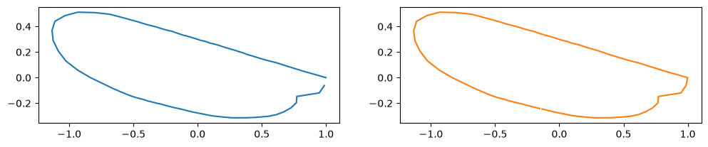
Changing the starting point#
The starting point (arclength parameter \(t = 0\) ) is often adjusted for aligning the outlines.
You can use the numpy.roll function for the purpose.
new_staring_points = np.array([rng.integers(0,len(coord)) for coord in coords], dtype=int)
coords_changed_start = [np.roll(coords[i], -new_staring_points[i], axis=0) for i in range(len(coords))]
idx = 0

fig, ax = plt.subplots(1,2, figsize=(12,7))
sns.lineplot(x=coords[idx][:,0], y=coords[idx][:,1], sort= False,estimator=None,ax=ax[0])
sns.lineplot(x=coords_changed_start[idx][:,0], y=coords_changed_start[idx][:,1],
             sort= False,color="C1",estimator=None,ax=ax[1])
ax[0].set_aspect('equal')
ax[1].set_aspect('equal')
print("starting point: ", new_staring_points[idx])
starting point: 67
See also
Elliptic Fourier Analysis for a complete EFA workflow
Harmonic-based Morphometrics for understanding harmonic-based normalization