Visualize Shape Variation

Display reconstructed shapes along component axes.

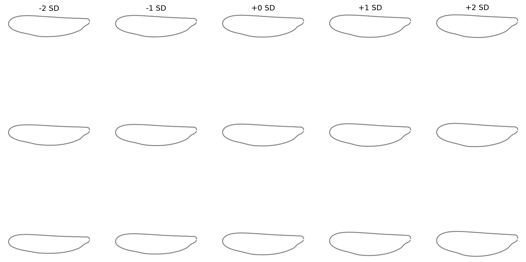
EFA outlines

import numpy as np
import matplotlib.pyplot as plt
from sklearn.decomposition import PCA

from ktch.datasets import load_outline_mosquito_wings
from ktch.harmonic import EllipticFourierAnalysis
from ktch.plot import shape_variation_plot

data = load_outline_mosquito_wings(as_frame=True)
coords = data.coords.to_numpy().reshape(-1, 100, 2)

efa = EllipticFourierAnalysis(n_harmonics=20)
coef = efa.fit_transform(coords)

pca = PCA(n_components=5).fit(coef)

fig = shape_variation_plot(
    pca,
    descriptor=efa,
    components=(0, 1, 2),
    sd_values=(-2, -1, 0, 1, 2),
)

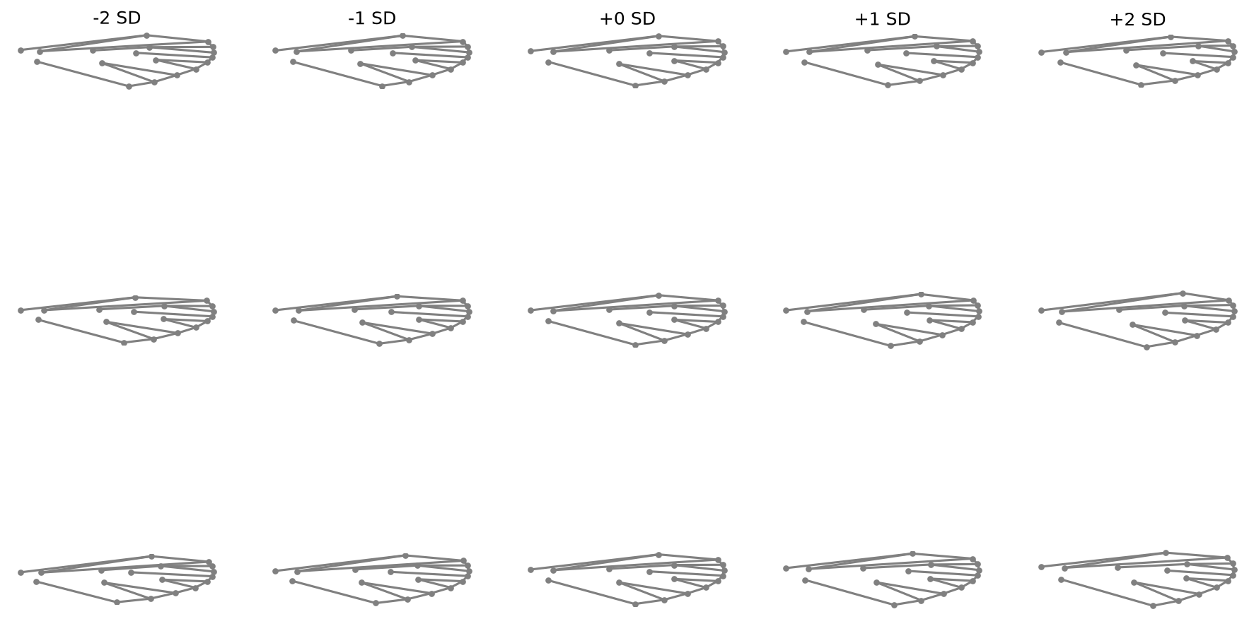
Landmarks with links

import pandas as pd
from ktch.datasets import load_landmark_mosquito_wings
from ktch.landmark import GeneralizedProcrustesAnalysis

data_lm = load_landmark_mosquito_wings(as_frame=True)
df_coords = (
    data_lm.coords.unstack()
    .swaplevel(1, 0, axis=1)
    .sort_index(axis=1)
)
df_coords.columns = [
    dim + "_" + str(idx) for idx, dim in df_coords.columns
]

gpa = GeneralizedProcrustesAnalysis().set_output(transform="pandas")
df_shapes = gpa.fit_transform(df_coords)

pca_lm = PCA(n_components=5).fit(df_shapes)

links = [
    [0, 1], [1, 2], [2, 3], [3, 4], [4, 5], [5, 6],
    [6, 7], [7, 8], [8, 9], [9, 10], [10, 11],
    [1, 12], [2, 12], [13, 14], [14, 3], [14, 4],
    [15, 5], [16, 6], [16, 7], [17, 8], [17, 9],
]

fig = shape_variation_plot(
    pca_lm,
    n_dim=2,
    links=links,
    components=(0, 1, 2),
    sd_values=(-2, -1, 0, 1, 2),
)

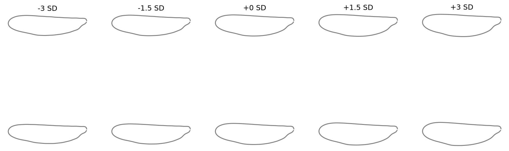
Select components and SD values

Show only specific components with custom SD steps:

fig = shape_variation_plot(
    pca,
    descriptor=efa,
    components=(0, 1),
    sd_values=(-3, -1.5, 0, 1.5, 3),
)

See also

• Visualize Morphospace for morphospace scatter plots with shape overlays

• Use Non-PCA Reducers for using KernelPCA and other non-PCA reducers

• Morphometric Visualization for the reconstruction pipeline design