Elliptic Fourier Analysis#
import numpy as np
import pandas as pd

import matplotlib.pyplot as plt
import seaborn as sns

from sklearn.decomposition import PCA

from ktch.datasets import load_outline_mosquito_wings
from ktch.harmonic import EllipticFourierAnalysis
from ktch.plot import explained_variance_ratio_plot
Load mosquito wing outline dataset#
from Rohlf and Archie 1984 Syst. Zool.
data_outline_mosquito_wings = load_outline_mosquito_wings(as_frame=True)
data_outline_mosquito_wings.coords
| x | y | ||
|---|---|---|---|
| specimen_id | coord_id | ||
| 1 | 0 | 0.99973 | 0.00000 |
| 1 | 0.81881 | 0.05151 | |
| 2 | 0.70063 | 0.08851 | |
| 3 | 0.61179 | 0.11670 | |
| 4 | 0.53226 | 0.13666 | |
| ... | ... | ... | ... |
| 126 | 95 | 0.68167 | -0.22149 |
| 96 | 0.76135 | -0.19548 | |
| 97 | 0.90752 | -0.17312 | |
| 98 | 0.95720 | -0.12093 | |
| 99 | 0.95964 | -0.06038 |
12600 rows × 2 columns
coords = data_outline_mosquito_wings.coords.to_numpy().reshape(-1, 100, 2)
fig, ax = plt.subplots()
sns.lineplot(x=coords[0][:, 0], y=coords[0][:, 1], sort=False, estimator=None, ax=ax)
ax.set_aspect("equal")

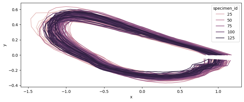
fig, ax = plt.subplots(figsize=(10, 10))
sns.lineplot(
    data=data_outline_mosquito_wings.coords,
    x="x",
    y="y",
    hue="specimen_id",
    sort=False,
    estimator=None,
    ax=ax,
)
ax.set_aspect("equal")
EFA#
efa = EllipticFourierAnalysis(n_harmonics=20)
coef = efa.fit_transform(coords)
PCA#
pca = PCA(n_components=12)
pcscores = pca.fit_transform(coef)
df_pca = pd.DataFrame(pcscores)
df_pca["specimen_id"] = [i for i in range(1, len(pcscores) + 1)]
df_pca = df_pca.set_index("specimen_id")
df_pca = df_pca.join(data_outline_mosquito_wings.meta)
df_pca = df_pca.rename(columns={i: ("PC" + str(i + 1)) for i in range(12)})
df_pca
| PC1 | PC2 | PC3 | PC4 | PC5 | PC6 | PC7 | PC8 | PC9 | PC10 | PC11 | PC12 | genus | |
|---|---|---|---|---|---|---|---|---|---|---|---|---|---|
| specimen_id | |||||||||||||
| 1 | 0.004277 | -0.019211 | 0.018697 | 0.000810 | -0.001363 | -0.015705 | 0.007489 | -0.000853 | -0.004332 | 0.000064 | -0.001233 | -0.000509 | AN |
| 2 | -0.034207 | 0.019829 | 0.000914 | 0.002444 | 0.004912 | 0.004622 | 0.002922 | -0.000719 | -0.008601 | -0.003872 | -0.002954 | 0.000656 | AN |
| 3 | -0.199464 | -0.031161 | -0.045073 | 0.008504 | -0.004950 | 0.006258 | 0.001273 | 0.004424 | -0.003027 | -0.000986 | 0.002781 | -0.001875 | AN |
| 4 | -0.248697 | 0.035792 | -0.019214 | -0.000370 | 0.007445 | -0.009597 | 0.004925 | 0.001945 | 0.001729 | -0.001801 | 0.001553 | -0.001683 | AN |
| 5 | 0.151898 | -0.057919 | -0.009257 | 0.009022 | 0.002941 | 0.009306 | 0.003443 | -0.001652 | -0.001026 | -0.004647 | -0.003179 | 0.000502 | AN |
| ... | ... | ... | ... | ... | ... | ... | ... | ... | ... | ... | ... | ... | ... |
| 122 | -0.084827 | 0.032089 | -0.023891 | 0.000607 | 0.007980 | -0.003300 | 0.000688 | 0.002950 | 0.003434 | -0.001497 | 0.002059 | 0.000181 | CX |
| 123 | -0.096891 | -0.043715 | 0.000709 | -0.007439 | -0.005802 | -0.003579 | 0.005781 | 0.000594 | 0.006692 | 0.001221 | -0.000017 | 0.001236 | CX |
| 124 | -0.119387 | 0.016518 | -0.031522 | -0.021842 | 0.001695 | 0.002130 | 0.002902 | 0.003965 | 0.000240 | -0.001915 | -0.001795 | 0.000932 | CX |
| 125 | -0.059915 | 0.046869 | 0.014093 | -0.002840 | 0.008363 | -0.001264 | 0.001011 | 0.000412 | 0.003208 | 0.004421 | -0.000136 | 0.000643 | CX |
| 126 | -0.035477 | 0.031945 | 0.008483 | -0.019398 | -0.002612 | 0.005169 | 0.004838 | -0.000205 | 0.002391 | -0.002302 | 0.000625 | -0.001556 | DE |
126 rows × 13 columns
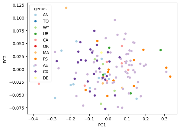
fig, ax = plt.subplots()
sns.scatterplot(data=df_pca, x="PC1", y="PC2", hue="genus", ax=ax, palette="Paired")
<Axes: xlabel='PC1', ylabel='PC2'>
Morphospace#
def get_pc_scores_for_morphospace(ax, num=5):
    xrange = np.linspace(ax.get_xlim()[0], ax.get_xlim()[1], num)
    yrange = np.linspace(ax.get_ylim()[0], ax.get_ylim()[1], num)
    return xrange, yrange


def plot_recon_morphs(
    pca,
    efa,
    fig,
    ax,
    n_PCs_xy=[1, 2],
    morph_num=3,
    morph_scale=1.0,
    morph_color="lightgray",
    morph_alpha=0.7,
):
    pc_scores_h, pc_scores_v = get_pc_scores_for_morphospace(ax, morph_num)
    print("PC_h: ", pc_scores_h, ", PC_v: ", pc_scores_v)
    for pc_score_h in pc_scores_h:
        for pc_score_v in pc_scores_v:
            pc_score = np.zeros(pca.n_components_)
            n_PC_h, n_PC_v = n_PCs_xy
            pc_score[n_PC_h - 1] = pc_score_h
            pc_score[n_PC_v - 1] = pc_score_v

            arr_coef = pca.inverse_transform([pc_score])

            ax_width = ax.get_window_extent().width
            fig_width = fig.get_window_extent().width
            fig_height = fig.get_window_extent().height
            morph_size = morph_scale * ax_width / (fig_width * morph_num)
            loc = ax.transData.transform((pc_score_h, pc_score_v))
            axins = fig.add_axes(
                [
                    loc[0] / fig_width - morph_size / 2,
                    loc[1] / fig_height - morph_size / 2,
                    morph_size,
                    morph_size,
                ],
                anchor="C",
            )

            coords = efa.inverse_transform(arr_coef)
            x = coords[0][:, 0]
            y = coords[0][:, 1]

            axins.plot(
                x.astype(float), y.astype(float), color=morph_color, alpha=morph_alpha
            )
            axins.axis("equal")
            axins.axis("off")
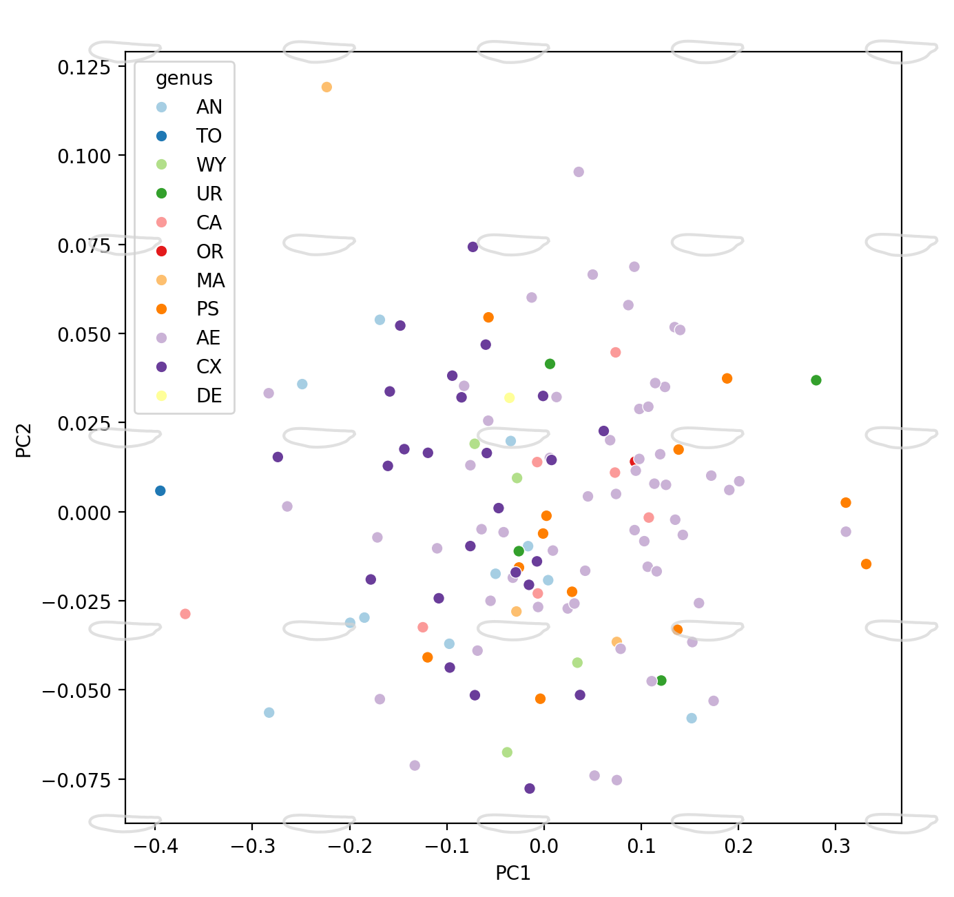
fig = plt.figure(figsize=(16, 16), dpi=200)

ax = fig.add_subplot(2, 2, 1)
sns.scatterplot(
    data=df_pca,
    x="PC1",
    y="PC2",
    hue="genus",
    hue_order=None,
    palette="Paired",
    ax=ax,
    legend=True,
)

plot_recon_morphs(pca, efa, morph_num=5, morph_scale=0.5, fig=fig, ax=ax)
PC_h: [-0.43098724 -0.23129168 -0.03159612 0.16809944 0.367795 ] , PC_v: [-0.08749144 -0.0333772 0.02073705 0.0748513 0.12896555]
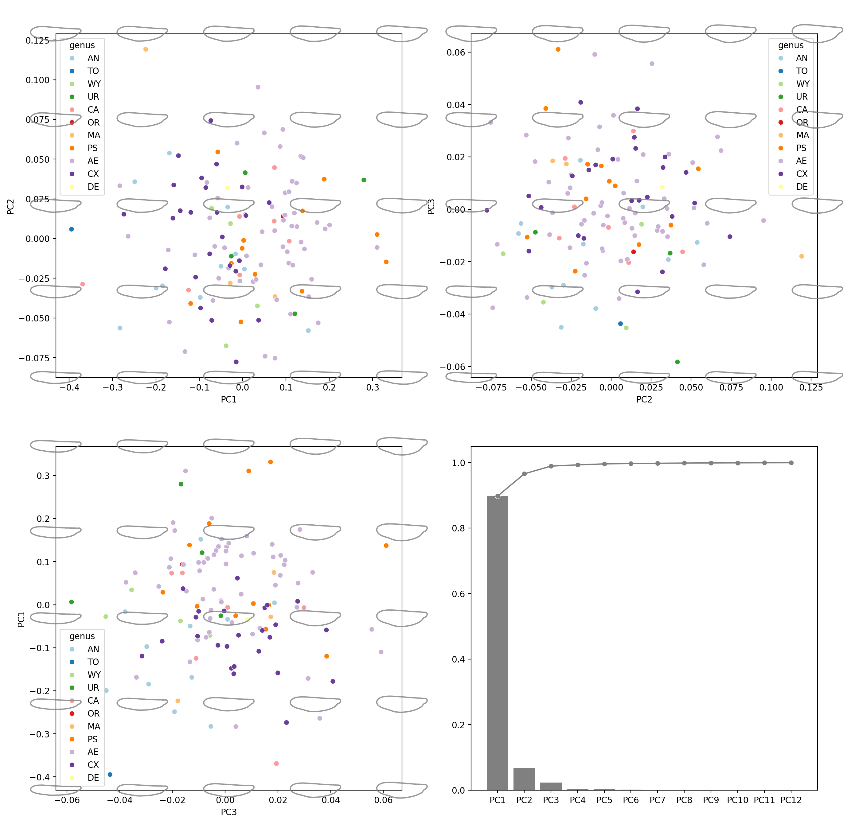
morph_num = 5
morph_scale = 0.8
morph_color = "gray"
morph_alpha = 0.8

hue_order = df_pca["genus"].unique()

fig = plt.figure(figsize=(16, 16), dpi=200)

#########
# PC1
#########
ax = fig.add_subplot(2, 2, 1)
sns.scatterplot(
    data=df_pca,
    x="PC1",
    y="PC2",
    hue="genus",
    hue_order=hue_order,
    palette="Paired",
    ax=ax,
    legend=True,
)

plot_recon_morphs(
    pca,
    efa,
    morph_num=5,
    morph_scale=morph_scale,
    morph_color=morph_color,
    morph_alpha=morph_alpha,
    fig=fig,
    ax=ax,
)

ax.patch.set_alpha(0)
ax.set(xlabel="PC1", ylabel="PC2")

print("PC1-PC2 done")

#########
# PC2
#########
ax = fig.add_subplot(2, 2, 2)
sns.scatterplot(
    data=df_pca,
    x="PC2",
    y="PC3",
    hue="genus",
    hue_order=hue_order,
    palette="Paired",
    ax=ax,
    legend=True,
)

plot_recon_morphs(
    pca,
    efa,
    morph_num=5,
    morph_scale=morph_scale,
    morph_color=morph_color,
    morph_alpha=morph_alpha,
    fig=fig,
    ax=ax,
    n_PCs_xy=[2, 3],
)

ax.patch.set_alpha(0)
ax.set(xlabel="PC2", ylabel="PC3")

print("PC2-PC3 done")

#########
# PC3
#########
ax = fig.add_subplot(2, 2, 3)
sns.scatterplot(
    data=df_pca,
    x="PC3",
    y="PC1",
    hue="genus",
    hue_order=hue_order,
    palette="Paired",
    ax=ax,
    legend=True,
)

plot_recon_morphs(
    pca,
    efa,
    morph_num=5,
    morph_scale=morph_scale,
    morph_color=morph_color,
    morph_alpha=morph_alpha,
    fig=fig,
    ax=ax,
    n_PCs_xy=[3, 1],
)

ax.patch.set_alpha(0)
ax.set(xlabel="PC3", ylabel="PC1")

print("PC3-PC1 done")

#########
# CCR
#########

ax = fig.add_subplot(2, 2, 4)
explained_variance_ratio_plot(pca, ax=ax, verbose=True)
PC_h:  [-0.43098724 -0.23129168 -0.03159612  0.16809944  0.367795  ] , PC_v:  [-0.08749144 -0.0333772   0.02073705  0.0748513   0.12896555]
PC1-PC2 done
PC_h:  [-0.08749144 -0.0333772   0.02073705  0.0748513   0.12896555] , PC_v:  [-0.06424967 -0.0314274   0.00139486  0.03421713  0.0670394 ]
PC2-PC3 done
PC_h:  [-0.06424967 -0.0314274   0.00139486  0.03421713  0.0670394 ] , PC_v:  [-0.43098724 -0.23129168 -0.03159612  0.16809944  0.367795  ]
PC3-PC1 done
Explained variance ratio:
['PC1 0.8973793082876147', 'PC2 0.06795826373299034', 'PC3 0.023626937292117314', 'PC4 0.003773503228718847', 'PC5 0.002928302449990927', 'PC6 0.001256061508173971', 'PC7 0.0007323203596517956', 'PC8 0.0005507118631158467', 'PC9 0.00043565710337472723', 'PC10 0.00030767134202518213', 'PC11 0.00022663508829736778', 'PC12 0.00015100902428697937']
Cumsum of Explained variance ratio:
['PC1 0.8973793082876147', 'PC2 0.965337572020605', 'PC3 0.9889645093127223', 'PC4 0.9927380125414411', 'PC5 0.995666314991432', 'PC6 0.9969223764996059', 'PC7 0.9976546968592577', 'PC8 0.9982054087223735', 'PC9 0.9986410658257482', 'PC10 0.9989487371677733', 'PC11 0.9991753722560707', 'PC12 0.9993263812803577']
<Axes: >