Elliptic Fourier Analysis

See also

For cases where automatic normalization is not suitable, see 2D Outline Registration.

import numpy as np
import pandas as pd

import matplotlib.pyplot as plt
import seaborn as sns

from sklearn.decomposition import PCA

from ktch.datasets import load_outline_mosquito_wings
from ktch.harmonic import EllipticFourierAnalysis
from ktch.plot import explained_variance_ratio_plot, morphospace_plot, shape_variation_plot

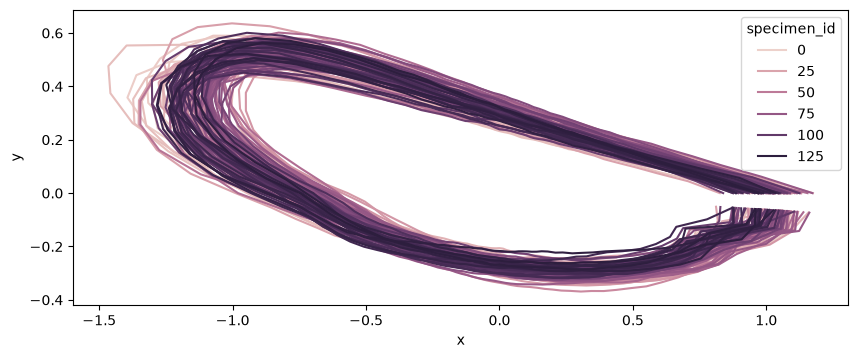
Load mosquito wing outline dataset

from Rohlf and Archie 1984 Syst. Zool.

data_outline_mosquito_wings = load_outline_mosquito_wings(as_frame=True)
data_outline_mosquito_wings.coords

		x	y
specimen_id	coord_id
0	0	0.99973	0.00000
	1	0.81881	0.05151
	2	0.70063	0.08851
	3	0.61179	0.11670
	4	0.53226	0.13666
...	...	...	...
125	95	0.68167	-0.22149
	96	0.76135	-0.19548
	97	0.90752	-0.17312
	98	0.95720	-0.12093
	99	0.95964	-0.06038

12600 rows × 2 columns

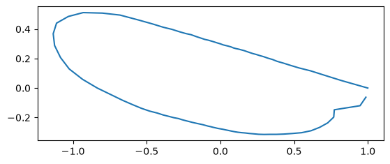
coords = data_outline_mosquito_wings.coords.to_numpy().reshape(-1, 100, 2)

fig, ax = plt.subplots()
sns.lineplot(x=coords[0][:, 0], y=coords[0][:, 1], sort=False, estimator=None, ax=ax)
ax.set_aspect("equal")

fig, ax = plt.subplots(figsize=(10, 10))
sns.lineplot(
    data=data_outline_mosquito_wings.coords,
    x="x",
    y="y",
    hue="specimen_id",
    sort=False,
    estimator=None,
    ax=ax,
)
ax.set_aspect("equal")

EFA

efa = EllipticFourierAnalysis(n_harmonics=20)

coef = efa.fit_transform(coords)

PCA

pca = PCA(n_components=12)
pcscores = pca.fit_transform(coef)

df_pca = pd.DataFrame(pcscores)
df_pca["specimen_id"] = list(range(len(pcscores)))
df_pca = df_pca.set_index("specimen_id")
df_pca = df_pca.join(data_outline_mosquito_wings.meta)
df_pca = df_pca.rename(columns={i: ("PC" + str(i + 1)) for i in range(12)})
df_pca

	PC1	PC2	PC3	PC4	PC5	PC6	PC7	PC8	PC9	PC10	PC11	PC12	genus
specimen_id
0	0.004277	-0.019211	0.018697	0.000810	-0.001363	-0.015705	0.007489	-0.000853	-0.004332	0.000064	-0.001233	-0.000509	AN
1	-0.034207	0.019829	0.000914	0.002444	0.004912	0.004622	0.002922	-0.000719	-0.008601	-0.003872	-0.002954	0.000656	AN
2	-0.199464	-0.031161	-0.045073	0.008504	-0.004950	0.006258	0.001273	0.004424	-0.003027	-0.000986	0.002781	-0.001875	AN
3	-0.248697	0.035792	-0.019214	-0.000370	0.007445	-0.009597	0.004925	0.001945	0.001729	-0.001801	0.001553	-0.001683	AN
4	0.151898	-0.057919	-0.009257	0.009022	0.002941	0.009306	0.003443	-0.001652	-0.001026	-0.004647	-0.003179	0.000502	AN
...	...	...	...	...	...	...	...	...	...	...	...	...	...
121	-0.084827	0.032089	-0.023891	0.000607	0.007980	-0.003300	0.000688	0.002950	0.003434	-0.001497	0.002059	0.000181	CX
122	-0.096891	-0.043715	0.000709	-0.007439	-0.005802	-0.003579	0.005781	0.000594	0.006692	0.001221	-0.000017	0.001236	CX
123	-0.119387	0.016518	-0.031522	-0.021842	0.001695	0.002130	0.002902	0.003965	0.000240	-0.001915	-0.001795	0.000932	CX
124	-0.059915	0.046869	0.014093	-0.002840	0.008363	-0.001264	0.001011	0.000412	0.003208	0.004421	-0.000136	0.000643	CX
125	-0.035477	0.031945	0.008483	-0.019398	-0.002612	0.005169	0.004838	-0.000205	0.002391	-0.002302	0.000625	-0.001556	DE

126 rows × 13 columns

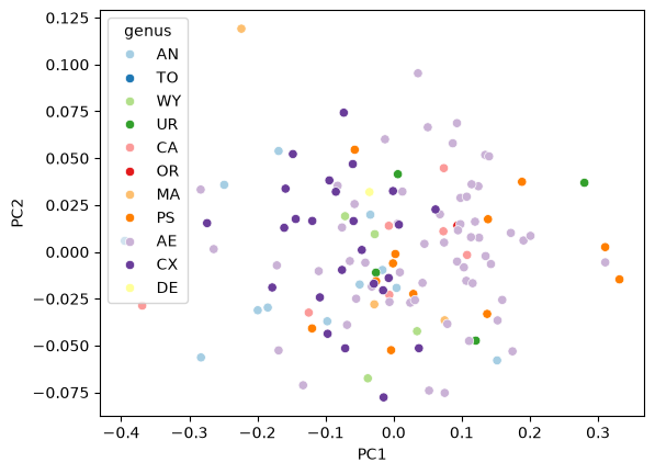
fig, ax = plt.subplots()
sns.scatterplot(data=df_pca, x="PC1", y="PC2", hue="genus", ax=ax, palette="Paired")

<Axes: xlabel='PC1', ylabel='PC2'>

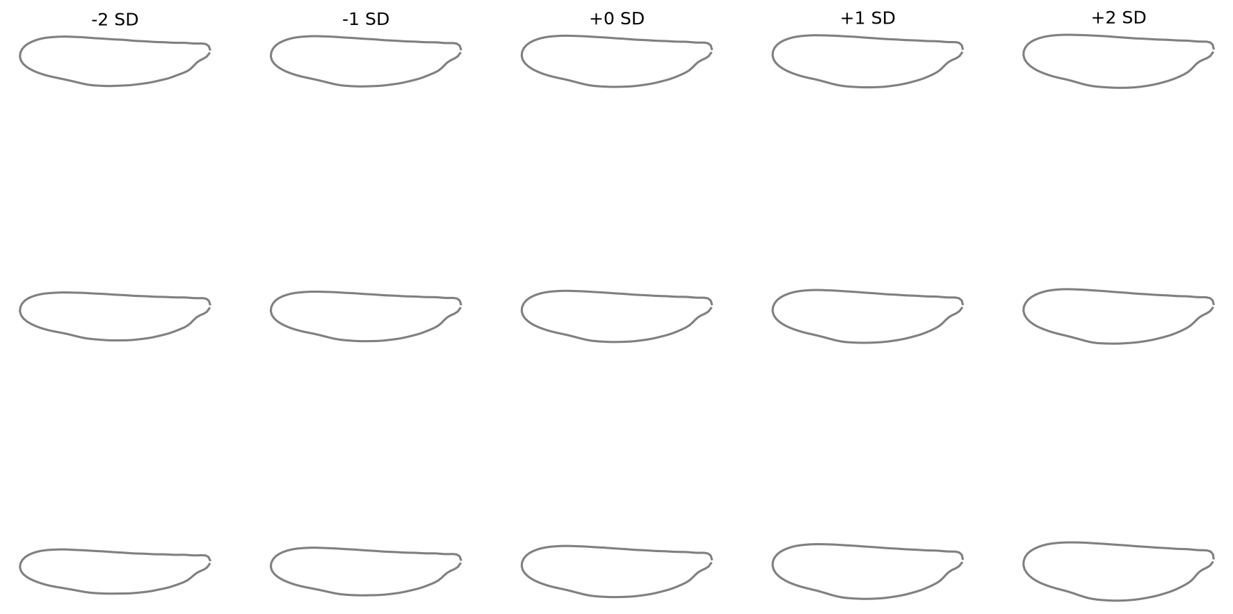
Shape variation along PC axes

fig = shape_variation_plot(
    pca,
    descriptor=efa,
    components=(0, 1, 2),
    sd_values=(-2, -1, 0, 1, 2),
)

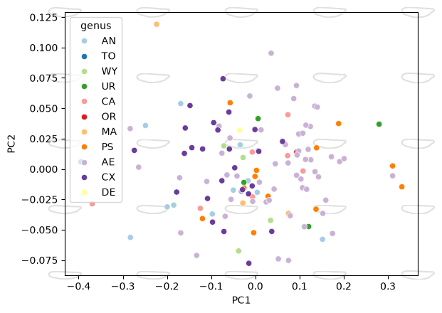
Morphospace

ax = morphospace_plot(
    data=df_pca,
    x="PC1", y="PC2", hue="genus",
    reducer=pca,
    descriptor=efa,
    palette="Paired",
    n_shapes=5,
    shape_scale=0.5,
)

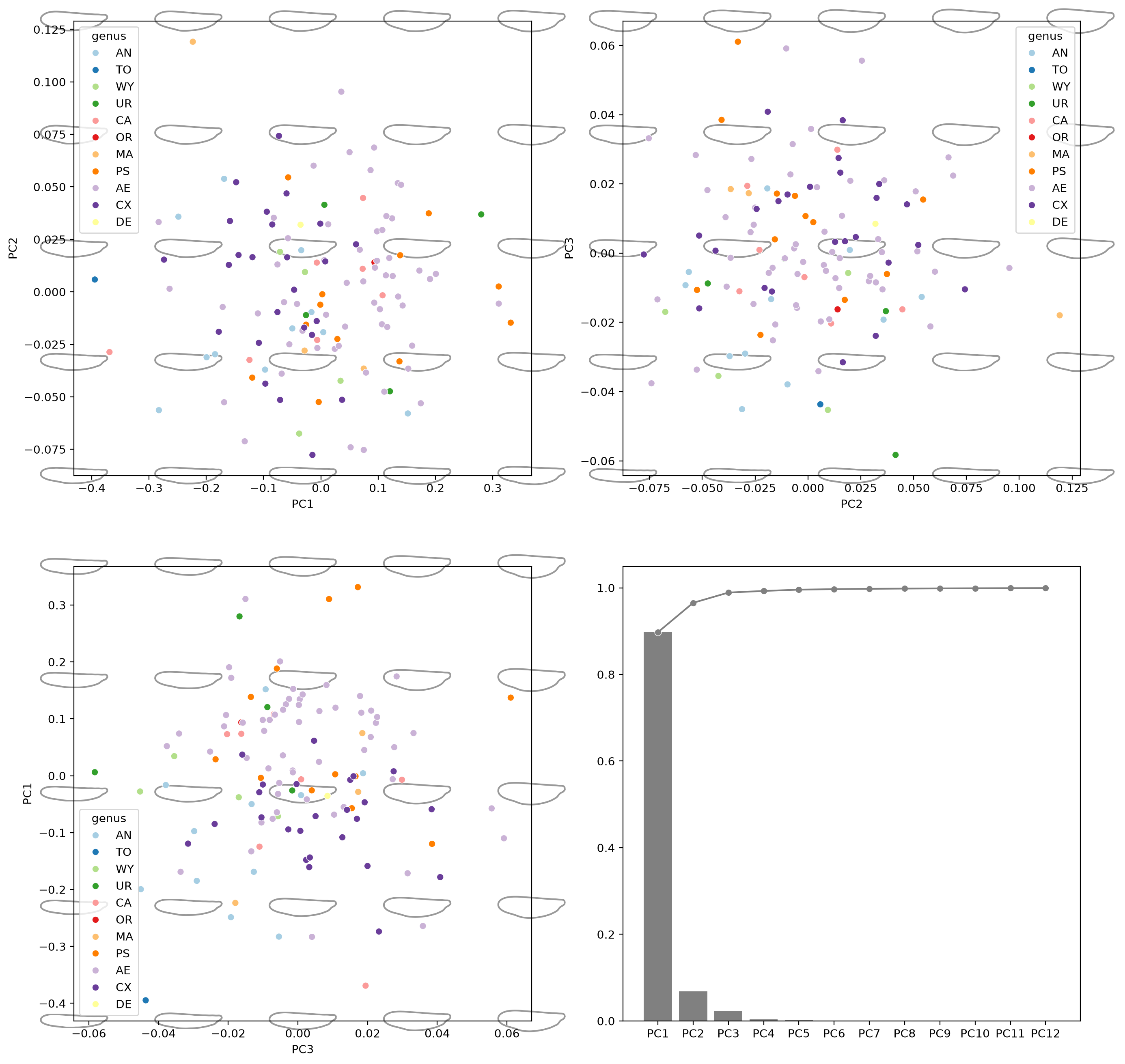
fig, axes = plt.subplots(2, 2, figsize=(16, 16), dpi=200)

for ax, (i, j) in zip(axes.flat[:3], [(0, 1), (1, 2), (2, 0)]):
    morphospace_plot(
        data=df_pca,
        x=f"PC{i + 1}", y=f"PC{j + 1}", hue="genus",
        reducer=pca,
        descriptor=efa,
        components=(i, j),
        palette="Paired",
        n_shapes=5,
        shape_color="gray",
        shape_scale=0.8,
        shape_alpha=0.8,
        ax=ax,
    )

explained_variance_ratio_plot(pca, ax=axes[1, 1])

<Axes: >