Generalized Procrustes analysis

import numpy as np
import pandas as pd

import matplotlib.pyplot as plt
from matplotlib.collections import LineCollection
import seaborn as sns

from sklearn.decomposition import PCA

from ktch.datasets import load_landmark_mosquito_wings
from ktch.landmark import GeneralizedProcrustesAnalysis
from ktch.plot import explained_variance_ratio_plot, morphospace_plot, shape_variation_plot

Load mosquito wing landmark dataset

from Rohlf and Slice 1990 Syst. Zool.

data_landmark_mosquito_wings = load_landmark_mosquito_wings(as_frame=True)
data_landmark_mosquito_wings.coords

		x	y
specimen_id	coord_id
0	0	-0.4933	0.0130
	1	-0.0777	0.0832
	2	0.2231	0.0861
	3	0.2641	0.0462
	4	0.2645	0.0261
...	...	...	...
126	13	-0.2028	0.0371
	14	0.0490	0.0347
	15	-0.0422	0.0204
	16	0.1004	-0.0180
	17	-0.1473	-0.0057

2286 rows × 2 columns

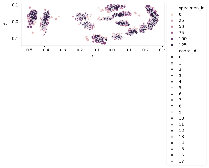
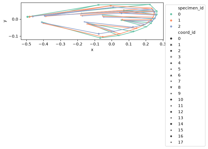
fig, ax = plt.subplots()
sns.scatterplot(
    data=data_landmark_mosquito_wings.coords,
    x="x",
    y="y",
    hue="specimen_id",
    style="coord_id",
    ax=ax,
)
ax.set_aspect("equal")
ax.legend(loc="upper left", bbox_to_anchor=(1, 1))

<matplotlib.legend.Legend at 0x7f7bf2091d50>

For applying generalized Procrustes analysis (GPA), we convert the configuration data into DataFrame of shape n_specimens x (n_landmarks*n_dim).

def configuration_plot(
    configuration_2d,
    x="x",
    y="y",
    links=None,
    ax=None,
    hue=None,
    hue_order=None,
    c="gray",
    palette=None,
    c_line="gray",
    style=None,
    s=10,
    alpha=1,
):
    if ax is None:
        fig = plt.figure()
        ax = fig.add_subplot(111)

    if links is None:
        links = []

    configuration = configuration_2d.reset_index()

    if hue is not None and hue_order is None:
        hue_order = configuration[hue].unique()

    color_map = None
    if hue is not None:
        if palette is not None:
            colors = sns.color_palette(palette, n_colors=len(hue_order))
            color_map = dict(zip(hue_order, colors))
        else:
            hue_dtype = configuration[hue].dtype
            if np.issubdtype(hue_dtype, np.number):
                cmap = sns.cubehelix_palette(as_cmap=True)
                hue_min, hue_max = min(hue_order), max(hue_order)
                color_map = {}
                for hue_val in hue_order:
                    if hue_max > hue_min:
                        norm_val = (hue_val - hue_min) / (hue_max - hue_min)
                    else:
                        norm_val = 0.5
                    color_map[hue_val] = cmap(norm_val)
            else:
                colors = sns.color_palette(n_colors=len(hue_order))
                color_map = dict(zip(hue_order, colors))

    if links:
        if hue is None:
            segments = []
            for link in links:
                link_data = configuration[configuration["coord_id"].isin(link)]
                if len(link_data) == 2:
                    coords = link_data[[x, y]].values
                    segments.append(coords)
            if segments:
                lc = LineCollection(segments, colors=c_line, alpha=alpha)
                ax.add_collection(lc)
        else:
            for specimen in hue_order:
                specimen_data = configuration[configuration[hue] == specimen]
                segments = []
                for link in links:
                    link_data = specimen_data[specimen_data["coord_id"].isin(link)]
                    if len(link_data) == 2:
                        coords = link_data[[x, y]].values
                        segments.append(coords)
                if segments:
                    lc = LineCollection(
                        segments, colors=[color_map[specimen]], alpha=alpha
                    )
                    ax.add_collection(lc)

        ax.autoscale_view()

    axis = sns.scatterplot(
        data=configuration,
        x=x,
        y=y,
        ax=ax,
        hue=hue,
        hue_order=hue_order,
        palette=palette,
        style=style,
        c=c,
        alpha=alpha,
        s=s,
    )

    if axis.legend_:
        sns.move_legend(ax, "upper left", bbox_to_anchor=(1, 1))

    ax.set_aspect("equal")

links = [
    [0, 1],
    [1, 2],
    [2, 3],
    [3, 4],
    [4, 5],
    [5, 6],
    [6, 7],
    [7, 8],
    [8, 9],
    [9, 10],
    [10, 11],
    [1, 12],
    [2, 12],
    [13, 14],
    [14, 3],
    [14, 4],
    [15, 5],
    [16, 6],
    [16, 7],
    [17, 8],
    [17, 9],
]

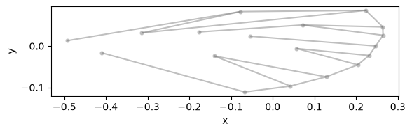
configuration_plot(
    data_landmark_mosquito_wings.coords.loc[0], links=links, alpha=0.5, s=20
)

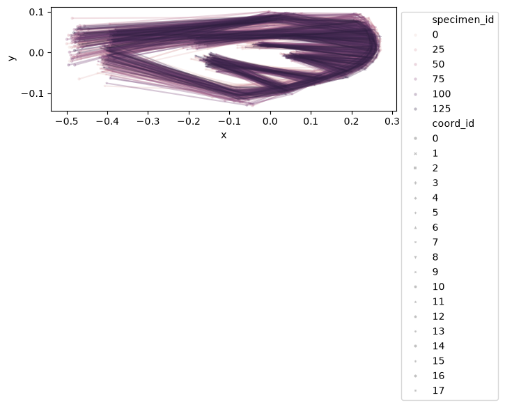
configuration_plot(
    data_landmark_mosquito_wings.coords,
    links=links,
    alpha=0.3,
    hue="specimen_id",
    style="coord_id",
)

configuration_plot(
    data_landmark_mosquito_wings.coords.loc[0:2],
    links=links,
    hue="specimen_id",
    style="coord_id",
    palette="Set2",
    s=30,
)

index = pd.MultiIndex.from_tuples(
    [(1, i) for i in data_landmark_mosquito_wings.coords.loc[1].index],
    names=["specimen_id", "coord_id"],
)
x2 = pd.DataFrame(
    data_landmark_mosquito_wings.coords.loc[1].to_numpy(),
    columns=["x", "y"],
    index=index,
)

data_landmark_mosquito_wings.coords.loc[0:2]

		x	y
specimen_id	coord_id
0	0	-0.4933	0.0130
	1	-0.0777	0.0832
	2	0.2231	0.0861
	3	0.2641	0.0462
	4	0.2645	0.0261
	5	0.2471	0.0003
	6	0.2311	-0.0228
	7	0.2040	-0.0452
	8	0.1282	-0.0742
	9	0.0424	-0.0966
	10	-0.0674	-0.1108
	11	-0.4102	-0.0163
	12	-0.3140	0.0318
	13	-0.1768	0.0341
	14	0.0715	0.0509
	15	-0.0540	0.0238
	16	0.0575	-0.0059
	17	-0.1401	-0.0240
1	0	-0.4814	0.0135
	1	-0.0058	0.0780
	2	0.2345	0.0644
	3	0.2460	0.0467
	4	0.2487	0.0281
	5	0.2430	0.0115
	6	0.2316	-0.0039
	7	0.1956	-0.0305
	8	0.1462	-0.0545
	9	0.0483	-0.0866
	10	-0.0520	-0.1047
	11	-0.4016	-0.0250
	12	-0.3868	0.0166
	13	-0.1808	0.0229
	14	0.0484	0.0405
	15	-0.0519	0.0164
	16	0.0623	-0.0047
	17	-0.1444	-0.0286
2	0	-0.4622	0.0159
	1	0.0089	0.0689
	2	0.2404	0.0545
	3	0.2501	0.0424
	4	0.2600	0.0230
	5	0.2541	0.0039
	6	0.2369	-0.0105
	7	0.1957	-0.0305
	8	0.1249	-0.0480
	9	0.0146	-0.0720
	10	-0.0758	-0.0865
	11	-0.4104	-0.0200
	12	-0.3919	0.0190
	13	-0.1724	0.0182
	14	0.0577	0.0344
	15	-0.0468	0.0115
	16	0.0766	-0.0079
	17	-0.1602	-0.0162

df_coords = (
    data_landmark_mosquito_wings.coords.unstack()
    .swaplevel(1, 0, axis=1)
    .sort_index(axis=1)
)
df_coords.columns = [
    dim + "_" + str(landmark_idx) for landmark_idx, dim in df_coords.columns
]
df_coords

	x_0	y_0	x_1	y_1	x_2	y_2	x_3	y_3	x_4	y_4	...	x_13	y_13	x_14	y_14	x_15	y_15	x_16	y_16	x_17	y_17
specimen_id
0	-0.4933	0.0130	-0.0777	0.0832	0.2231	0.0861	0.2641	0.0462	0.2645	0.0261	...	-0.1768	0.0341	0.0715	0.0509	-0.0540	0.0238	0.0575	-0.0059	-0.1401	-0.0240
1	-0.4814	0.0135	-0.0058	0.0780	0.2345	0.0644	0.2460	0.0467	0.2487	0.0281	...	-0.1808	0.0229	0.0484	0.0405	-0.0519	0.0164	0.0623	-0.0047	-0.1444	-0.0286
2	-0.4622	0.0159	0.0089	0.0689	0.2404	0.0545	0.2501	0.0424	0.2600	0.0230	...	-0.1724	0.0182	0.0577	0.0344	-0.0468	0.0115	0.0766	-0.0079	-0.1602	-0.0162
3	-0.4534	-0.0028	-0.0318	0.0738	0.2423	0.0808	0.2627	0.0559	0.2654	0.0322	...	-0.1536	0.0150	0.0617	0.0436	-0.0549	0.0217	0.0705	-0.0031	-0.1507	-0.0273
4	-0.4926	-0.0212	-0.0260	0.0708	0.2347	0.0679	0.2398	0.0584	0.2415	0.0355	...	-0.1374	0.0154	0.0762	0.0457	-0.0313	0.0170	0.0880	0.0037	-0.1318	-0.0278
...	...	...	...	...	...	...	...	...	...	...	...	...	...	...	...	...	...	...	...	...	...
122	-0.4703	-0.0009	0.0011	0.0805	0.2146	0.0747	0.2348	0.0585	0.2453	0.0350	...	-0.1624	0.0193	0.0557	0.0467	-0.0272	0.0190	0.0718	-0.0052	-0.1583	-0.0251
123	-0.4725	0.0441	0.0318	0.0808	0.2382	0.0419	0.2504	0.0237	0.2492	0.0019	...	-0.1724	0.0390	0.0667	0.0418	-0.0108	0.0205	0.0548	-0.0049	-0.1546	-0.0115
124	-0.4697	0.0196	0.0007	0.0850	0.2228	0.0760	0.2485	0.0540	0.2548	0.0319	...	-0.1816	0.0213	0.0376	0.0408	-0.0073	0.0137	0.0592	-0.0103	-0.1531	-0.0300
125	-0.4620	0.0204	0.0082	0.0893	0.2061	0.0797	0.2374	0.0529	0.2457	0.0306	...	-0.1876	0.0241	0.0279	0.0403	-0.0425	0.0145	0.0729	-0.0123	-0.1460	-0.0269
126	-0.4570	0.0468	-0.0090	0.0753	0.2381	0.0463	0.2556	0.0275	0.2614	0.0064	...	-0.2028	0.0371	0.0490	0.0347	-0.0422	0.0204	0.1004	-0.0180	-0.1473	-0.0057

127 rows × 36 columns

GPA

gpa = GeneralizedProcrustesAnalysis().set_output(transform="pandas")

df_shapes = gpa.fit_transform(df_coords)
df_shapes

	x_0	y_0	x_1	y_1	x_2	y_2	x_3	y_3	x_4	y_4	...	x_13	y_13	x_14	y_14	x_15	y_15	x_16	y_16	x_17	y_17
specimen_id
0	-0.488913	0.021159	-0.075651	0.083813	0.222655	0.081656	0.262641	0.041408	0.262701	0.021471	...	-0.174735	0.036786	0.071747	0.049290	-0.053145	0.024519	0.056916	-0.006796	-0.139317	-0.021437
1	-0.479850	0.030667	-0.002995	0.078029	0.236289	0.055873	0.247131	0.037801	0.249161	0.019145	...	-0.179578	0.029304	0.049746	0.038675	-0.051194	0.018213	0.062000	-0.006922	-0.145098	-0.023383
2	-0.461238	0.021194	0.009668	0.068674	0.240606	0.051631	0.250150	0.039440	0.259809	0.019959	...	-0.171907	0.020150	0.057987	0.033671	-0.046599	0.012014	0.076367	-0.008775	-0.160124	-0.014331
3	-0.451582	0.021733	-0.027671	0.075199	0.245617	0.067345	0.264582	0.041450	0.265988	0.017707	...	-0.152122	0.023242	0.063790	0.040074	-0.053488	0.024575	0.070026	-0.006899	-0.151522	-0.019031
4	-0.491092	0.019428	-0.020015	0.072475	0.238724	0.048169	0.243009	0.038313	0.242816	0.015425	...	-0.135231	0.026596	0.079447	0.039142	-0.029701	0.019466	0.087717	-0.003550	-0.133219	-0.016779
...	...	...	...	...	...	...	...	...	...	...	...	...	...	...	...	...	...	...	...	...	...
122	-0.468838	0.028646	0.006143	0.080164	0.218584	0.060969	0.237700	0.043553	0.246690	0.019469	...	-0.160671	0.029436	0.058442	0.043044	-0.025929	0.020642	0.071228	-0.009699	-0.159374	-0.015077
123	-0.473804	0.016670	0.027045	0.082425	0.235150	0.055559	0.248370	0.038112	0.248433	0.016300	...	-0.174200	0.028931	0.064108	0.045546	-0.011957	0.019822	0.054939	-0.001719	-0.153528	-0.020407
124	-0.468449	0.032047	0.002958	0.084844	0.224473	0.069955	0.249549	0.047306	0.255251	0.025073	...	-0.180752	0.026088	0.038626	0.039732	-0.006925	0.013867	0.058834	-0.011863	-0.153659	-0.025890
125	-0.459471	0.036434	0.011277	0.088662	0.208061	0.072197	0.238303	0.044411	0.245792	0.021909	...	-0.186025	0.030549	0.029190	0.039168	-0.041832	0.015925	0.072178	-0.014794	-0.146368	-0.021701
126	-0.457745	0.025260	-0.012492	0.074647	0.235186	0.057309	0.253512	0.039387	0.260281	0.018625	...	-0.203892	0.027493	0.047226	0.036891	-0.043017	0.018365	0.100931	-0.013236	-0.146563	-0.012573

127 rows × 36 columns

We create a DataFrame, called df_shapes_vis, of shape (n_specimens*n_landmarks) x n_dim to visualize the aligned shapes.

df_shapes_vis = df_shapes.copy()
df_shapes_vis.columns = pd.MultiIndex.from_tuples(
    [
        [int(landmark_idx), dim]
        for dim, landmark_idx in [idx.split("_") for idx in df_shapes_vis.columns]
    ],
    names=["coord_id", "dim"],
)
df_shapes_vis.sort_index(axis=1, inplace=True)
df_shapes_vis = df_shapes_vis.swaplevel(0, 1, axis=1).stack(level=1, future_stack=True)
df_shapes_vis

	dim	x	y
specimen_id	coord_id
0	0	-0.488913	0.021159
	1	-0.075651	0.083813
	2	0.222655	0.081656
	3	0.262641	0.041408
	4	0.262701	0.021471
...	...	...	...
126	13	-0.203892	0.027493
	14	0.047226	0.036891
	15	-0.043017	0.018365
	16	0.100931	-0.013236
	17	-0.146563	-0.012573

2286 rows × 2 columns

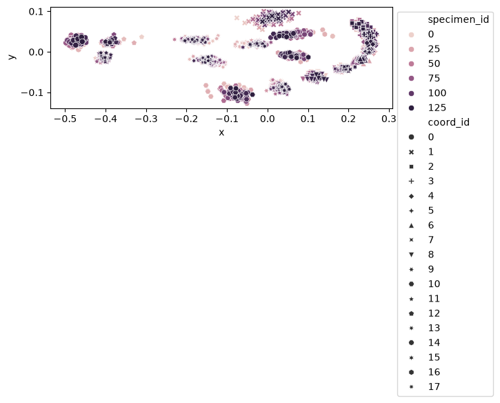
fig, ax = plt.subplots()
sns.scatterplot(
    data=df_shapes_vis, x="x", y="y", hue="specimen_id", style="coord_id", ax=ax
)
ax.set_aspect("equal")
ax.legend(loc="upper left", bbox_to_anchor=(1, 1))

<matplotlib.legend.Legend at 0x7f7bac210290>

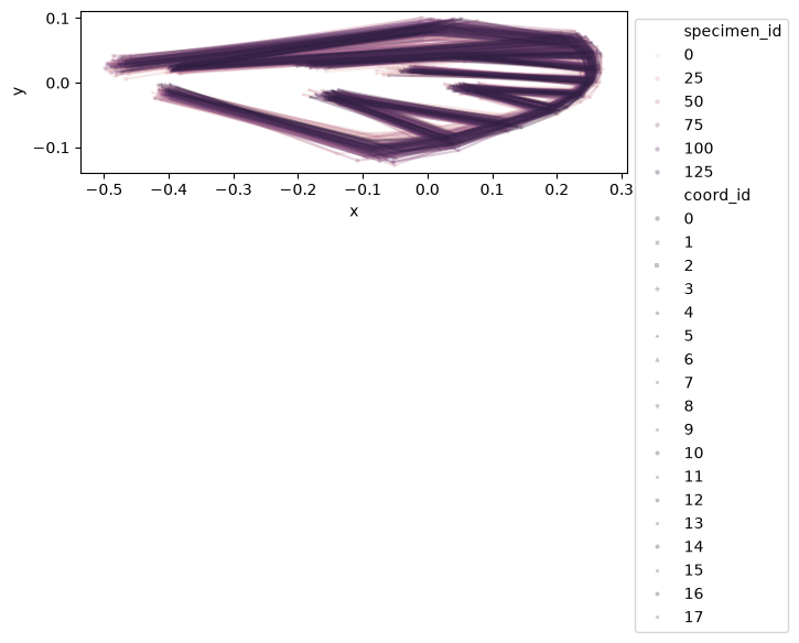
configuration_plot(
    df_shapes_vis, links=links, alpha=0.3, hue="specimen_id", style="coord_id"
)

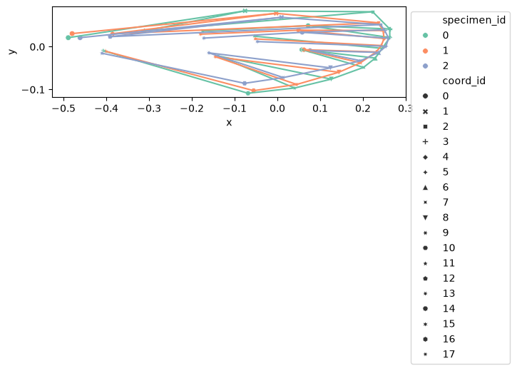
configuration_plot(
    df_shapes_vis.loc[0:2],
    links=links,
    hue="specimen_id",
    style="coord_id",
    palette="Set2",
    s=30,
)

PCA

pca = PCA(n_components=10).set_output(transform="pandas")
df_pca = pca.fit_transform(df_shapes)

df_pca = df_pca.join(data_landmark_mosquito_wings.meta)
df_pca

	pca0	pca1	pca2	pca3	pca4	pca5	pca6	pca7	pca8	pca9	genus
specimen_id
0	-0.003856	-0.093210	0.029908	0.049589	-0.007598	0.042657	-0.005370	0.010359	-0.011595	0.034991	AN
1	-0.029857	-0.023434	0.006114	-0.017268	-0.014229	0.014271	0.013344	0.021849	-0.011211	0.005069	AN
2	-0.012572	-0.019728	-0.034610	-0.025665	-0.005116	-0.017905	0.008511	-0.004312	0.001597	0.009884	AN
3	-0.001652	-0.049890	-0.034137	-0.001013	0.019706	-0.010102	-0.001692	-0.010425	0.021595	-0.006472	AN
4	0.026869	-0.032989	0.010228	-0.051852	0.016741	0.023749	0.015917	-0.000273	-0.013100	0.012755	AN
...	...	...	...	...	...	...	...	...	...	...	...
122	-0.007864	-0.009853	-0.006369	-0.026082	-0.025424	0.013786	-0.009967	-0.018669	0.000513	-0.005515	CX
123	-0.005360	0.014451	-0.014347	-0.013199	0.000102	0.001379	-0.002919	-0.009755	-0.020409	-0.017790	CX
124	-0.030056	0.000885	0.013455	0.000542	-0.008940	0.008503	-0.021390	-0.014563	-0.003408	-0.010083	CX
125	-0.048757	-0.000199	0.024147	-0.029841	-0.040190	0.013335	0.000598	0.016086	0.018985	0.004560	DE
126	-0.017155	-0.030018	-0.001935	-0.014438	-0.014540	-0.035565	-0.011888	0.017324	-0.009739	0.012342	DE

127 rows × 11 columns

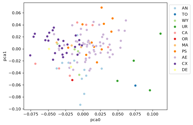
fig, ax = plt.subplots()
sns.scatterplot(data=df_pca, x="pca0", y="pca1", hue="genus", palette="Paired", ax=ax)
ax.legend(loc="upper left", bbox_to_anchor=(1, 1))

<matplotlib.legend.Legend at 0x7f7ba7bc5c10>

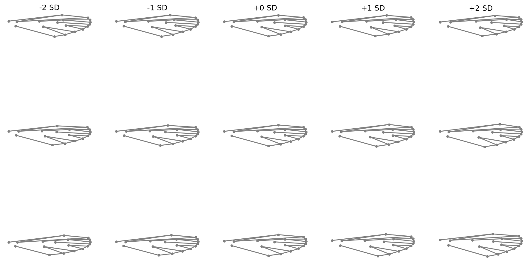
Shape variation along PC axes

fig = shape_variation_plot(
    pca,
    n_dim=2,
    links=links,
    components=(0, 1, 2),
    sd_values=(-2, -1, 0, 1, 2),
)

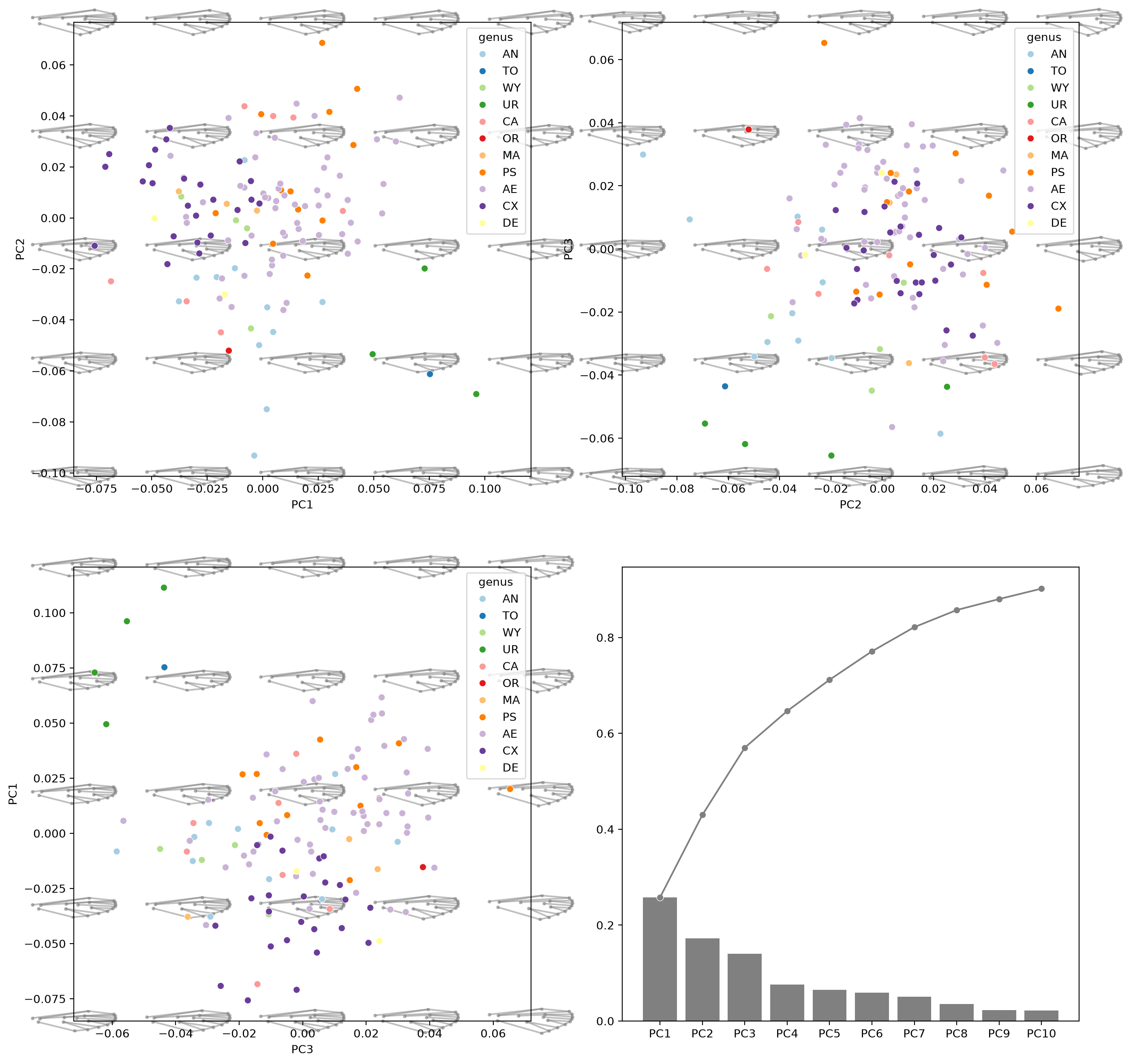
Morphospace

fig, axes = plt.subplots(2, 2, figsize=(16, 16), dpi=200)

for ax, (i, j) in zip(axes.flat[:3], [(0, 1), (1, 2), (2, 0)]):
    morphospace_plot(
        data=df_pca,
        x=f"pca{i}", y=f"pca{j}", hue="genus",
        reducer=pca,
        n_dim=2,
        components=(i, j),
        links=links,
        palette="Paired",
        n_shapes=5,
        shape_color="gray",
        shape_scale=1.0,
        shape_alpha=0.5,
        ax=ax,
        s=5,
    )
    ax.set(xlabel=f"PC{i + 1}", ylabel=f"PC{j + 1}")

explained_variance_ratio_plot(pca, ax=axes[1, 1])

<Axes: >