Semilandmark analysis

import numpy as np
import pandas as pd

import matplotlib.pyplot as plt
from matplotlib.collections import LineCollection
import seaborn as sns

from sklearn.decomposition import PCA

from ktch.datasets import load_landmark_trilobite_cephala
from ktch.landmark import GeneralizedProcrustesAnalysis, combine_landmarks_and_curves
from ktch.plot import explained_variance_ratio_plot

Load trilobite cephalon dataset

This dataset contains 2D landmark and semilandmark configurations of trilobite cephala (head shields). Each specimen has 16 fixed landmarks and 4 curves with semilandmarks (12, 20, 20, and 20 points respectively).

data = load_landmark_trilobite_cephala()
landmarks = data.landmarks
curves = data.curves

print("landmarks shape:", landmarks.shape)
print("number of curves per specimen:", len(curves[0]))
for i, c in enumerate(curves[0]):
    print(f"  curve {i}: {c.shape[0]} points")

landmarks shape: (300, 16, 2)
number of curves per specimen: 4
  curve 0: 12 points
  curve 1: 20 points
  curve 2: 20 points
  curve 3: 20 points

df_meta = pd.DataFrame(data.meta)
df_meta.head()

	genus	species	ref_pic	locality	formation	min_age	max_age	format	has_scale
1020_Liu_1977	Hunanolenus	Hunanolenus genalatus	Liu 1977	Hunan	Huaqiao	Paibian	Paibian	xml	True
1023_Liu_1977	Huangshiaspis	Huangshiaspis transversus	Liu 1977	Fenghuang area	Tingziguan	Jiangshanian	Jiangshanian	xml	True
AMF27749	Weania	Weania semicircularis	Vanderlaan y Ebach 2015	Glen William Road	Flagstaff	Middle Visean	Upper Visean	xml	True
AMNH_28896	Eldredgeops	Eldredgeops raNAmilleri	Burton and Eldredge 1974	NaN	NaN	Eifelian	NaN	tps	True
AMNH_28902	Viaphacops	Viaphacops stummi	Eldredge 1973	NaN	NaN	Eifelian	NaN	tps	True

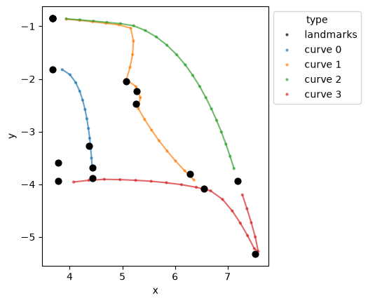
Visualize raw data

def configuration_plot(
    configuration_2d,
    x="x",
    y="y",
    links=None,
    ax=None,
    hue=None,
    hue_order=None,
    c="gray",
    palette=None,
    c_line="gray",
    style=None,
    s=10,
    alpha=1,
):
    if ax is None:
        fig = plt.figure()
        ax = fig.add_subplot(111)

    if links is None:
        links = []

    configuration = configuration_2d.reset_index()

    if hue is not None and hue_order is None:
        hue_order = configuration[hue].unique()

    color_map = None
    if hue is not None:
        if palette is not None:
            colors = sns.color_palette(palette, n_colors=len(hue_order))
            color_map = dict(zip(hue_order, colors))
        else:
            hue_dtype = configuration[hue].dtype
            if np.issubdtype(hue_dtype, np.number):
                cmap = sns.cubehelix_palette(as_cmap=True)
                hue_min, hue_max = min(hue_order), max(hue_order)
                color_map = {}
                for hue_val in hue_order:
                    if hue_max > hue_min:
                        norm_val = (hue_val - hue_min) / (hue_max - hue_min)
                    else:
                        norm_val = 0.5
                    color_map[hue_val] = cmap(norm_val)
            else:
                colors = sns.color_palette(n_colors=len(hue_order))
                color_map = dict(zip(hue_order, colors))

    if links:
        if hue is None:
            segments = []
            for link in links:
                link_data = configuration[configuration["coord_id"].isin(link)]
                if len(link_data) == 2:
                    coords = link_data[[x, y]].values
                    segments.append(coords)
            if segments:
                lc = LineCollection(segments, colors=c_line, alpha=alpha)
                ax.add_collection(lc)
        else:
            for specimen in hue_order:
                specimen_data = configuration[configuration[hue] == specimen]
                segments = []
                for link in links:
                    link_data = specimen_data[specimen_data["coord_id"].isin(link)]
                    if len(link_data) == 2:
                        coords = link_data[[x, y]].values
                        segments.append(coords)
                if segments:
                    lc = LineCollection(
                        segments, colors=[color_map[specimen]], alpha=alpha
                    )
                    ax.add_collection(lc)

        ax.autoscale_view()

    axis = sns.scatterplot(
        data=configuration,
        x=x,
        y=y,
        ax=ax,
        hue=hue,
        hue_order=hue_order,
        palette=palette,
        style=style,
        c=c,
        alpha=alpha,
        s=s,
    )

    if axis.legend_:
        sns.move_legend(ax, "upper left", bbox_to_anchor=(1, 1))

    ax.set_aspect("equal")

Plot a single specimen, distinguishing fixed landmarks from curve semilandmarks.

specimen_idx = 0

fig, ax = plt.subplots(figsize=(6, 6))

# Fixed landmarks
lm = landmarks[specimen_idx]
ax.scatter(lm[:, 0], lm[:, 1], c="black", s=40, zorder=3, label="landmarks")

# Curve semilandmarks
curve_colors = ["tab:blue", "tab:orange", "tab:green", "tab:red"]
for i, curve in enumerate(curves[specimen_idx]):
    ax.plot(curve[:, 0], curve[:, 1], "o-", color=curve_colors[i], markersize=3, alpha=0.7, label=f"curve {i} ({curve.shape[0]} pts)")

ax.set_aspect("equal")
ax.legend(loc="upper left", bbox_to_anchor=(1, 1))
ax.set_title("Specimen 0: landmarks and curve semilandmarks")

Text(0.5, 1.0, 'Specimen 0: landmarks and curve semilandmarks')

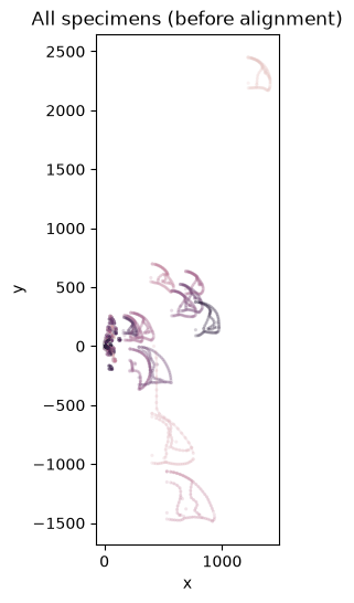
Plot all specimens overlaid before alignment.

fig, ax = plt.subplots(figsize=(6, 6))

for i in range(landmarks.shape[0]):
    lm = landmarks[i]
    ax.scatter(lm[:, 0], lm[:, 1], c="gray", s=5, alpha=0.2)
    for curve in curves[i]:
        ax.plot(curve[:, 0], curve[:, 1], c="gray", alpha=0.1, linewidth=0.5)

ax.set_aspect("equal")
ax.set_title("All specimens (before alignment)")

Text(0.5, 1.0, 'All specimens (before alignment)')

Combine landmarks and curves

combine_landmarks_and_curves() merges the fixed landmarks and curve semilandmarks into a single configuration array and generates the slider matrix that defines the sliding topology.

The curve_landmarks parameter specifies which landmarks anchor each curve. Each curve’s semilandmarks slide along the tangent direction, with the specified landmarks serving as fixed endpoints.

combined, slider_matrix, curve_info = combine_landmarks_and_curves(
    landmarks,
    curves,
    curve_landmarks=data.curve_landmarks,
)
print("combined shape:", combined.shape)
print("slider_matrix shape:", slider_matrix.shape)
print("curve_info:", curve_info)

combined shape: (300, 88, 2)
slider_matrix shape: (72, 3)
curve_info: {'n_landmarks': 16, 'n_curve_points': 72, 'curve_offsets': [16, 28, 48, 68], 'curve_lengths': [12, 20, 20, 20]}

The slider matrix has shape (n_sliders, 3) where each row is [before_index, slider_index, after_index]. All semilandmarks are included in the slider matrix. For curve endpoints, the before/after neighbor is the anchoring landmark.

print("First 5 rows of slider_matrix:")
print(slider_matrix[:5])

First 5 rows of slider_matrix:
[[ 1 16 17]
 [16 17 18]
 [17 18 19]
 [18 19 20]
 [19 20 21]]

Reshape the combined array to 2D (n_specimens, n_points * n_dim) for GPA input. Specimens containing NaN values are excluded.

X = combined.reshape(combined.shape[0], -1)

nan_mask = np.any(np.isnan(X), axis=1)
print(f"Specimens with NaN: {nan_mask.sum()} / {X.shape[0]}")

X_clean = X[~nan_mask]
df_meta_clean = df_meta[~nan_mask].reset_index(drop=True)
print(f"Specimens used for analysis: {X_clean.shape[0]}")

Specimens with NaN: 15 / 300
Specimens used for analysis: 285

GPA with semilandmark sliding

Pass the curves parameter to GeneralizedProcrustesAnalysis to enable semilandmark sliding during Procrustes superimposition. Semilandmarks slide along their curve tangent directions to minimize bending energy.

The tol parameter controls convergence tolerance for the iterative GPA algorithm.

gpa = GeneralizedProcrustesAnalysis(n_dim=2, curves=slider_matrix, tol=1e-3)
shapes = gpa.fit_transform(X_clean)
print("shapes shape:", shapes.shape)

shapes shape: (285, 176)

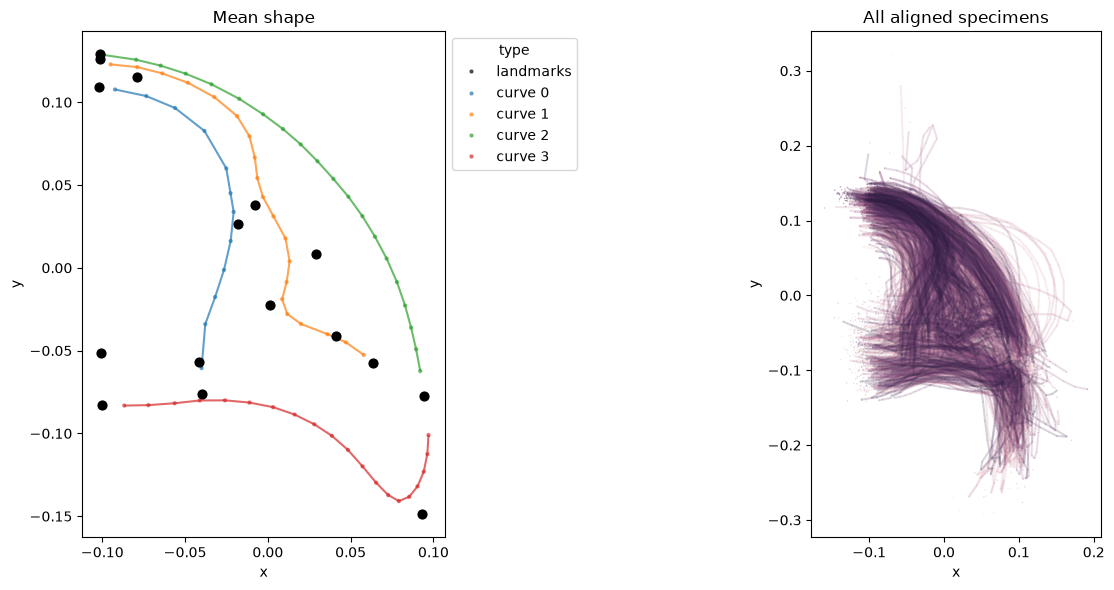
Visualize the aligned shapes.

n_points = combined.shape[1]
n_dim = 2

fig, axes = plt.subplots(1, 2, figsize=(14, 6))

# Mean shape
mean_shape = shapes.mean(axis=0).reshape(n_points, n_dim)
axes[0].scatter(mean_shape[:16, 0], mean_shape[:16, 1], c="black", s=40, zorder=3)
offset = 16
for i, length in enumerate(curve_info["curve_lengths"]):
    start = offset
    end = offset + length
    axes[0].plot(
        mean_shape[start:end, 0], mean_shape[start:end, 1],
        "o-", color=curve_colors[i], markersize=3, alpha=0.7,
    )
    offset = end
axes[0].set_aspect("equal")
axes[0].set_title("Mean shape")

# All aligned specimens
for i in range(shapes.shape[0]):
    specimen = shapes[i].reshape(n_points, n_dim)
    axes[1].scatter(specimen[:, 0], specimen[:, 1], c="gray", s=1, alpha=0.1)
axes[1].set_aspect("equal")
axes[1].set_title("All aligned specimens")

plt.tight_layout()

PCA

pca = PCA(n_components=10)
pc_scores = pca.fit_transform(shapes)

df_pca = pd.DataFrame(
    pc_scores,
    columns=[f"PC{i+1}" for i in range(pc_scores.shape[1])],
)
df_pca = df_pca.join(df_meta_clean[["genus"]])
df_pca.head()

	PC1	PC2	PC3	PC4	PC5	PC6	PC7	PC8	PC9	PC10	genus
0	-0.125228	-0.162647	0.004561	0.050726	0.019523	0.050510	-0.016427	0.043711	0.002174	-0.025951	Hunanolenus
1	-0.041252	-0.236899	0.140655	0.112496	0.036621	0.002261	0.001618	0.024187	-0.056088	0.014121	Huangshiaspis
2	0.009868	-0.111546	-0.027055	-0.132076	0.009976	-0.019524	0.101439	-0.009635	0.039078	-0.067129	Weania
3	0.142255	0.099790	0.069591	-0.034382	-0.008973	0.026952	0.003910	0.059150	-0.012461	0.021385	Eldredgeops
4	0.088966	0.111502	0.055935	-0.030005	0.049822	0.041755	0.008725	0.068558	-0.035017	0.035339	Viaphacops

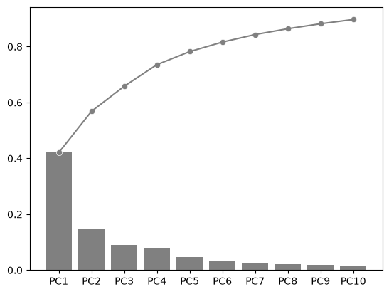
fig, ax = plt.subplots()
explained_variance_ratio_plot(pca, ax=ax, verbose=True)

Explained variance ratio:
['PC1 0.42068741054454406', 'PC2 0.14777776920504326', 'PC3 0.08970444170632054', 'PC4 0.07734131043972747', 'PC5 0.04661834564482889', 'PC6 0.034164966274203346', 'PC7 0.026888923778912794', 'PC8 0.02088629426179321', 'PC9 0.01773085494508937', 'PC10 0.015285218556972435']
Cumsum of Explained variance ratio:
['PC1 0.42068741054454406', 'PC2 0.5684651797495873', 'PC3 0.6581696214559078', 'PC4 0.7355109318956353', 'PC5 0.7821292775404642', 'PC6 0.8162942438146676', 'PC7 0.8431831675935805', 'PC8 0.8640694618553737', 'PC9 0.8818003168004631', 'PC10 0.8970855353574355']

<Axes: >

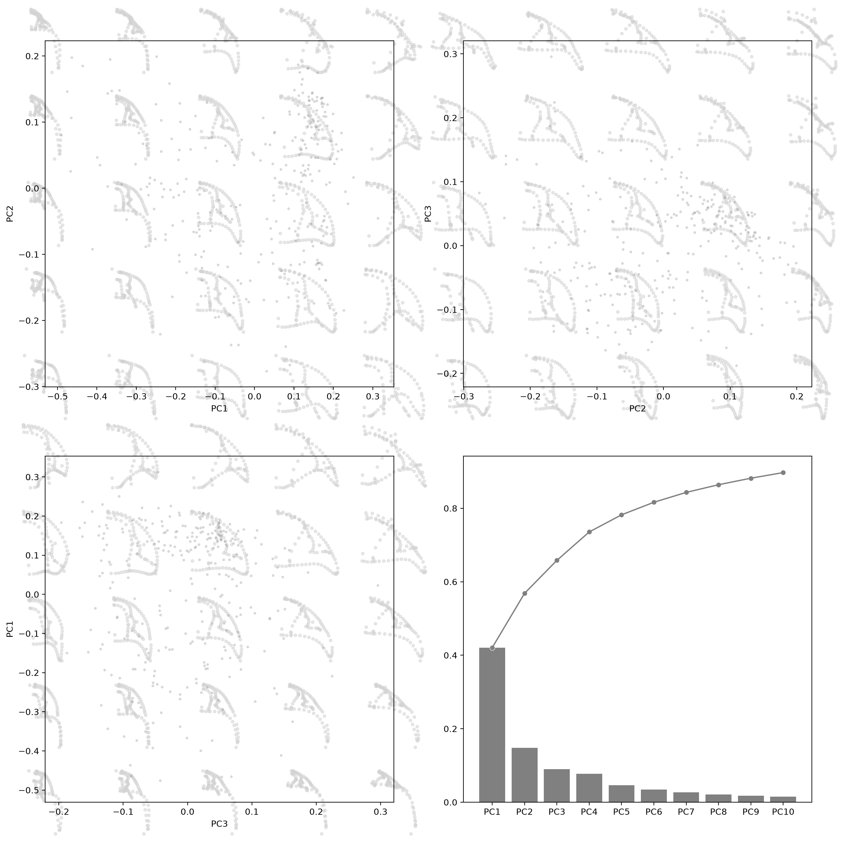
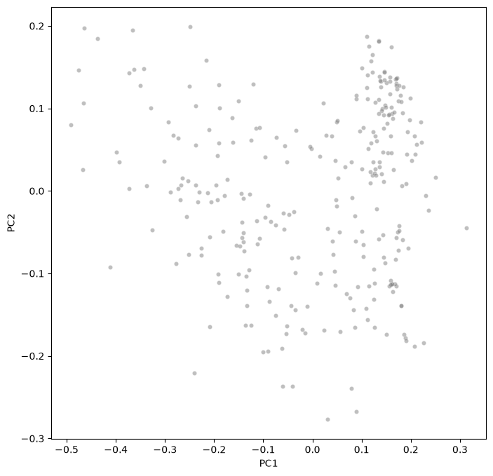
Morphospace visualization

fig, ax = plt.subplots(figsize=(8, 8))
sns.scatterplot(
    data=df_pca,
    x="PC1",
    y="PC2",
    ax=ax,
    c="gray",
    alpha=0.5,
    s=20,
)
ax.set(xlabel="PC1", ylabel="PC2")

[Text(0.5, 0, 'PC1'), Text(0, 0.5, 'PC2')]

Reconstruct shapes at grid positions in PC1–PC2 space.

def get_pc_scores_for_morphospace(ax, num=5):
    xrange = np.linspace(ax.get_xlim()[0], ax.get_xlim()[1], num)
    yrange = np.linspace(ax.get_ylim()[0], ax.get_ylim()[1], num)
    return xrange, yrange


def plot_recon_morphs(
    pca,
    fig,
    ax,
    n_PCs_xy=[1, 2],
    morph_num=3,
    morph_alpha=1.0,
    morph_scale=1.0,
    links=[],
):
    pc_scores_h, pc_scores_v = get_pc_scores_for_morphospace(ax, morph_num)
    for pc_score_h in pc_scores_h:
        for pc_score_v in pc_scores_v:
            pc_score = np.zeros(pca.n_components_)
            n_PC_h, n_PC_v = n_PCs_xy
            pc_score[n_PC_h - 1] = pc_score_h
            pc_score[n_PC_v - 1] = pc_score_v

            arr_shapes = pca.inverse_transform([pc_score])
            arr_shapes = arr_shapes.reshape(-1, 2)

            df_shapes = pd.DataFrame(arr_shapes, columns=["x", "y"])
            df_shapes["coord_id"] = [i for i in range(len(df_shapes))]
            df_shapes = df_shapes.set_index("coord_id")

            ax_width = ax.get_window_extent().width
            fig_width = fig.get_window_extent().width
            fig_height = fig.get_window_extent().height
            morph_size = morph_scale * ax_width / (fig_width * morph_num)
            loc = ax.transData.transform((pc_score_h, pc_score_v))

            axins = fig.add_axes(
                [
                    loc[0] / fig_width - morph_size / 2,
                    loc[1] / fig_height - morph_size / 2,
                    morph_size,
                    morph_size,
                ],
                anchor="C",
            )
            configuration_plot(df_shapes, links=links, ax=axins, alpha=morph_alpha)

            axins.axis("off")

morph_num = 5
morph_scale = 1.0
morph_alpha = 0.5

fig = plt.figure(figsize=(16, 16), dpi=200)

#########
# PC1-PC2
#########
ax = fig.add_subplot(2, 2, 1)
sns.scatterplot(
    data=df_pca,
    x="PC1",
    y="PC2",
    ax=ax,
    c="gray",
    alpha=0.3,
    s=10,
)

plot_recon_morphs(
    pca,
    morph_num=5,
    morph_scale=morph_scale,
    morph_alpha=0.5,
    fig=fig,
    ax=ax,
)

ax.patch.set_alpha(0)
ax.set(xlabel="PC1", ylabel="PC2")

#########
# PC2-PC3
#########
ax = fig.add_subplot(2, 2, 2)
sns.scatterplot(
    data=df_pca,
    x="PC2",
    y="PC3",
    ax=ax,
    c="gray",
    alpha=0.3,
    s=10,
)

plot_recon_morphs(
    pca,
    morph_num=5,
    morph_scale=morph_scale,
    morph_alpha=0.5,
    fig=fig,
    ax=ax,
    n_PCs_xy=[2, 3],
)

ax.patch.set_alpha(0)
ax.set(xlabel="PC2", ylabel="PC3")

#########
# PC3-PC1
#########
ax = fig.add_subplot(2, 2, 3)
sns.scatterplot(
    data=df_pca,
    x="PC3",
    y="PC1",
    ax=ax,
    c="gray",
    alpha=0.3,
    s=10,
)

plot_recon_morphs(
    pca,
    morph_num=5,
    morph_scale=morph_scale,
    morph_alpha=0.5,
    fig=fig,
    ax=ax,
    n_PCs_xy=[3, 1],
)

ax.patch.set_alpha(0)
ax.set(xlabel="PC3", ylabel="PC1")

#########
# Explained variance
#########
ax = fig.add_subplot(2, 2, 4)
explained_variance_ratio_plot(pca, ax=ax, verbose=True)

Explained variance ratio:
['PC1 0.42068741054454406', 'PC2 0.14777776920504326', 'PC3 0.08970444170632054', 'PC4 0.07734131043972747', 'PC5 0.04661834564482889', 'PC6 0.034164966274203346', 'PC7 0.026888923778912794', 'PC8 0.02088629426179321', 'PC9 0.01773085494508937', 'PC10 0.015285218556972435']
Cumsum of Explained variance ratio:
['PC1 0.42068741054454406', 'PC2 0.5684651797495873', 'PC3 0.6581696214559078', 'PC4 0.7355109318956353', 'PC5 0.7821292775404642', 'PC6 0.8162942438146676', 'PC7 0.8431831675935805', 'PC8 0.8640694618553737', 'PC9 0.8818003168004631', 'PC10 0.8970855353574355']

<Axes: >