2D Outline Extraction from Images

This tutorial shows how to extract outlines from images based on conventional image processing methods for use with ktch’s Elliptic Fourier Analysis (EFA).

Prerequisites

# !pip install ktch[data] opencv-python  # Uncomment if needed

Step 1: Load Images

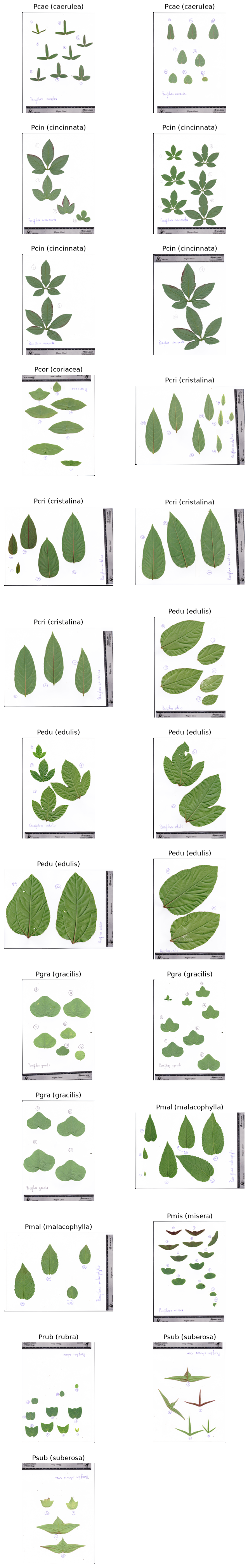
We use the Passiflora leaf scan dataset bundled with ktch: 25 flatbed scan images of 10 Passiflora species spanning simple elliptical to deeply lobed leaf forms. Each image contains multiple leaves from one plant individual, arranged from tip (youngest) to base (oldest). This dataset is a subset of the Passiflora leaf scan data from Chitwood & Otoni (2017) (data: Chitwood & Otoni, 2016). See data.DESCR for full details.

import numpy as np
import cv2 as cv
import matplotlib.pyplot as plt

from ktch.datasets import load_image_passiflora_leaves

Show definition: plot_images()

Hide definition: plot_images()

def plot_images(images, title_suffix="", cmap=None, outlines_per_image=None, labels=None, n_cols=2):
    """Plot images in a grid, optionally with outlines overlaid."""
    n_images = len(images)
    n_rows = (n_images + n_cols - 1) // n_cols

    fig, axes = plt.subplots(n_rows, n_cols, figsize=(4 * n_cols, 4 * n_rows))
    axes = axes.flatten()

    for i, ax in enumerate(axes):
        if i < n_images:
            label = labels[i] if labels is not None else f"Image {i+1}"
            if outlines_per_image is not None:
                ax.imshow(images[i])
                outlines = outlines_per_image[i]
                colors = plt.cm.tab10(np.linspace(0, 1, max(len(outlines), 1)))
                for j, outline in enumerate(outlines):
                    ax.plot(outline[:, 0], outline[:, 1], "-", linewidth=2, color=colors[j])
                ax.set_title(f"{label}: {len(outlines)} leaves")
            else:
                ax.imshow(images[i], cmap=cmap)
                title = label
                if title_suffix:
                    title += f" ({title_suffix})"
                ax.set_title(title)
        ax.axis("off")
    plt.tight_layout()

data = load_image_passiflora_leaves(as_frame=True)

print(f"Number of images: {len(data.images)}")
print(f"Species: {data.meta['species'].nunique()}")
print()
print(data.meta[["abbreviation", "species"]].value_counts().sort_index())

Downloading data from 'https://pub-c1d6dba6c94843f88f0fd096d19c0831.r2.dev/datasets/image_passiflora_leaves/v2/image_passiflora_leaves.zip' to file '/home/runner/.cache/ktch-data/image_passiflora_leaves/v2/image_passiflora_leaves.zip'.

Number of images: 25
Species: 10

abbreviation  species     
Pcae          caerulea        2
Pcin          cincinnata      4
Pcor          coriacea        1
Pcri          cristalina      4
Pedu          edulis          5
Pgra          gracilis        3
Pmal          malacophylla    2
Pmis          misera          1
Prub          rubra           1
Psub          suberosa        2
Name: count, dtype: int64

labels = [
    f"{row.abbreviation} ({row.species})"
    for _, row in data.meta.iterrows()
]
plot_images(data.images, labels=labels)

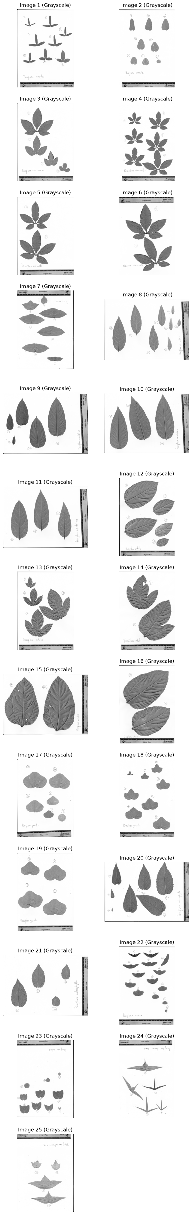
Step 2: Convert to Grayscale

images_gray = [cv.cvtColor(img, cv.COLOR_RGB2GRAY) for img in data.images]

plot_images(images_gray, "Grayscale", cmap="gray")

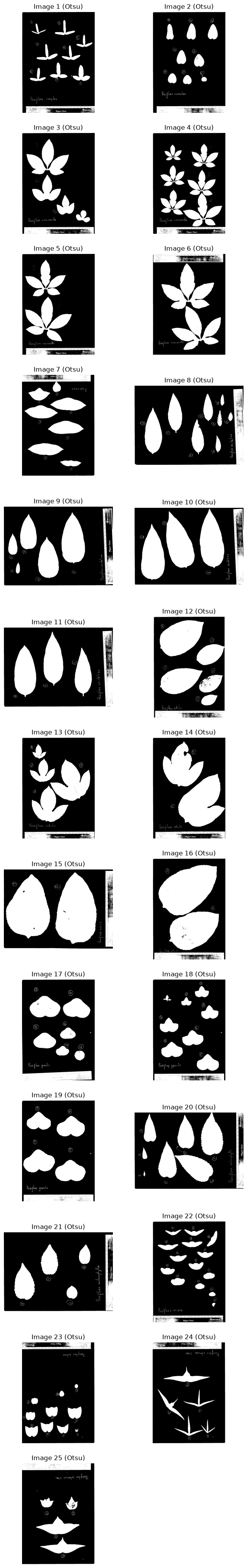
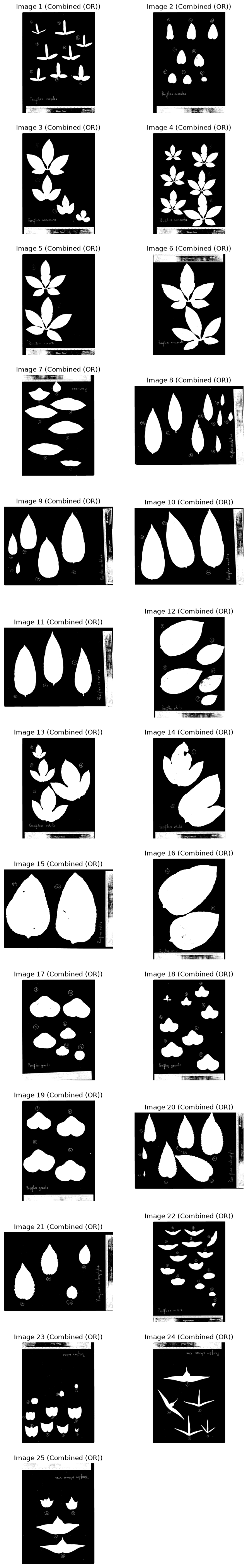
Step 3: Binarize the Image

We combine two binarization methods with OR to capture leaves that are either darker than the background or green in color.

Otsu’s thresholding

Automatically finds a threshold based on brightness histogram.

images_binary_otsu = []

for img_gray in images_gray:
    _, binary_otsu = cv.threshold(
        img_gray, 0, 255, cv.THRESH_BINARY_INV + cv.THRESH_OTSU
    )
    images_binary_otsu.append(binary_otsu)

plot_images(images_binary_otsu, "Otsu", cmap="gray")

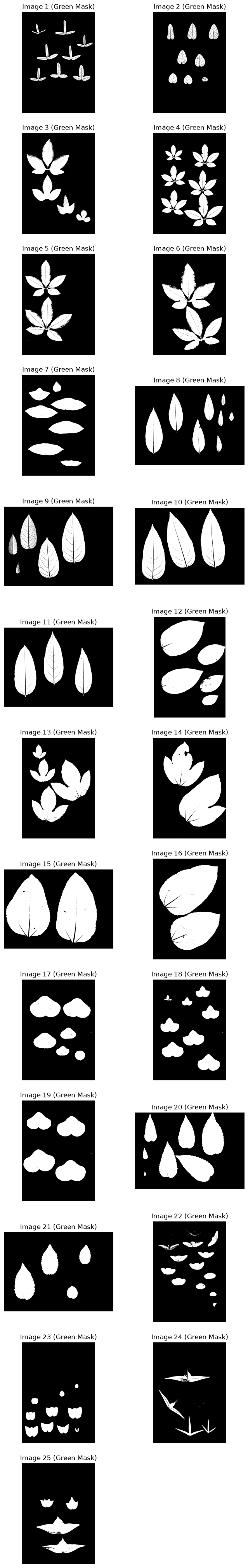
Green mask in HSV

Targets green hues with sufficient saturation and value.

hue_min, hue_max = 30, 90
sat_min, val_min = 40, 40

images_binary_green = []

for img_rgb in data.images:
    img_hsv = cv.cvtColor(img_rgb, cv.COLOR_RGB2HSV)
    lower_green = np.array([hue_min, sat_min, val_min])
    upper_green = np.array([hue_max, 255, 255])
    binary_green = cv.inRange(img_hsv, lower_green, upper_green)
    images_binary_green.append(binary_green)

plot_images(images_binary_green, "Green Mask", cmap="gray")

Combine with OR

images_binary = [
    cv.bitwise_or(otsu, green)
    for otsu, green in zip(images_binary_otsu, images_binary_green)
]

plot_images(images_binary, "Combined (OR)", cmap="gray")

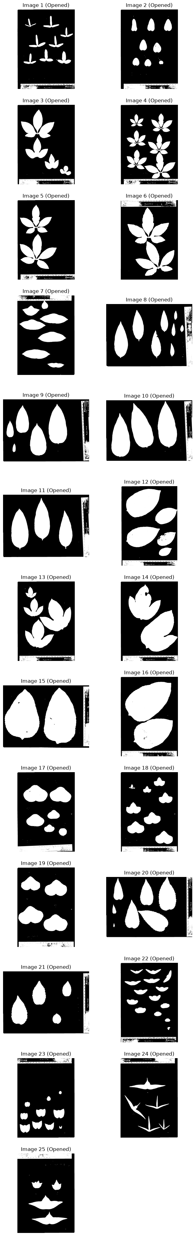
Step 4: Morphological Opening

Remove small noise with morphological opening.

kernel_size = 5
kernel = cv.getStructuringElement(cv.MORPH_ELLIPSE, (kernel_size, kernel_size))

images_opened = [
    cv.morphologyEx(img_binary, cv.MORPH_OPEN, kernel)
    for img_binary in images_binary
]

plot_images(images_opened, "Opened", cmap="gray")

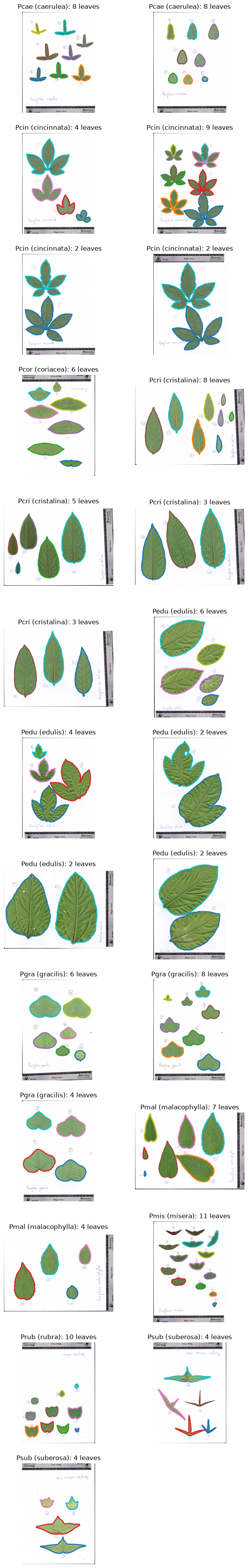
Step 5: Extract Outlines

Extract contours and filter by area and color.

Warning

This simple pipeline does not work perfectly for all images.

For example, deeply lobed species like P. cincinnata may have individual leaflets detected as separate leaves, and pale-colored leaves in P. edulis scans may be partially merged with the background, producing jagged outlines.

These cases require species-specific tuning or more advanced segmentation methods, but are left as-is here to illustrate typical failure cases.

Color filter function

def is_green_region(img_rgb, contour, hue_range=(30, 90), min_green_ratio=0.5):
    """Check if the contour region contains enough green pixels."""
    mask = np.zeros(img_rgb.shape[:2], dtype=np.uint8)
    cv.drawContours(mask, [contour], 0, 255, -1)

    region_pixels = img_rgb[mask == 255]
    if len(region_pixels) == 0:
        return False

    region_rgb = region_pixels.reshape(-1, 1, 3)
    region_hsv = cv.cvtColor(region_rgb, cv.COLOR_RGB2HSV).reshape(-1, 3)

    h, s, v = region_hsv[:, 0], region_hsv[:, 1], region_hsv[:, 2]
    is_green = (h >= hue_range[0]) & (h <= hue_range[1]) & (s >= 40) & (v >= 40)

    return np.sum(is_green) / len(region_pixels) >= min_green_ratio

Filter parameters

min_area = 50
hue_range = (30, 90)
min_green_ratio = 0.5

Extract and filter contours

all_outlines = []
outlines_per_image = []

for idx, img_opened in enumerate(images_opened):
    img_rgb = data.images[idx]

    contours, _ = cv.findContours(
        img_opened, cv.RETR_EXTERNAL, cv.CHAIN_APPROX_NONE
    )

    contours_filtered = [
        c for c in contours
        if cv.contourArea(c) >= min_area
        and is_green_region(img_rgb, c, hue_range, min_green_ratio)
    ]

    outlines = [c[:, 0, :].astype(np.float64) for c in contours_filtered]
    outlines_per_image.append(outlines)
    all_outlines.extend(outlines)

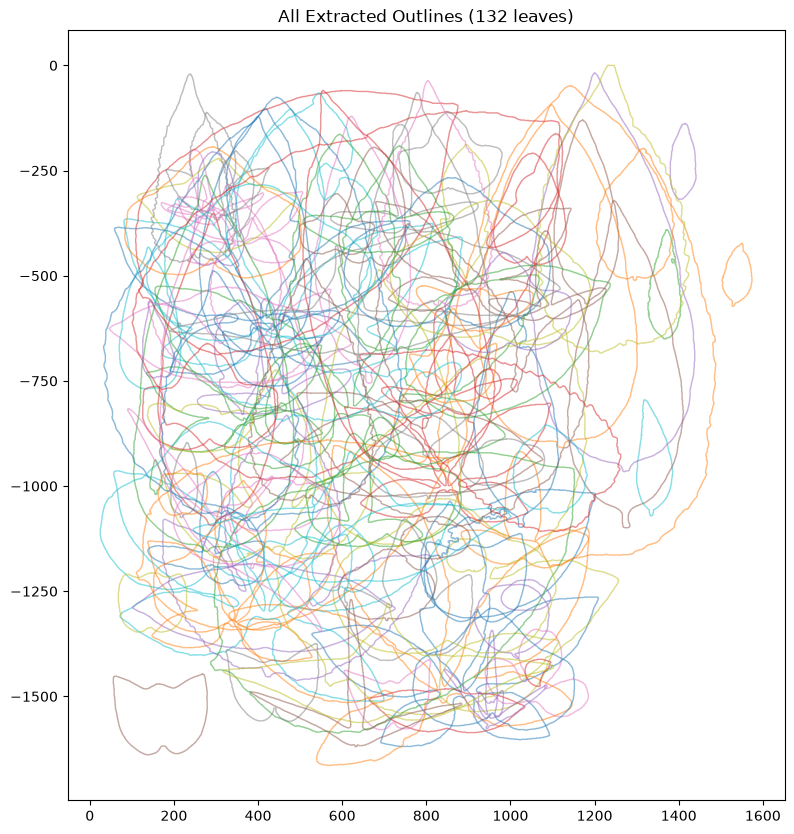
print(f"Total: {len(all_outlines)} outlines")

Total: 132 outlines

plot_images(data.images, outlines_per_image=outlines_per_image, labels=labels)

if len(all_outlines) > 0:
    fig, ax = plt.subplots(figsize=(10, 10))
    for outline in all_outlines:
        ax.plot(outline[:, 0], -outline[:, 1], alpha=0.5, linewidth=1)
    ax.set_aspect("equal")
    ax.set_title(f"All Extracted Outlines ({len(all_outlines)} leaves)")
    plt.tight_layout()
else:
    print("No outlines to plot")

Step 6: Verify Output Format

The output format is compatible with ktch’s EllipticFourierAnalysis.

print(f"Type: {type(all_outlines)}")
print(f"Number of specimens: {len(all_outlines)}")

if len(all_outlines) == 0:
    print("\nWarning: No outlines detected. Try adjusting parameters:")
    print("  - Decrease min_area")
    print("  - Adjust hue_range for your object color")
    print("  - Decrease min_green_ratio")
else:
    print(f"Shape of first outline: {all_outlines[0].shape}")

Type: <class 'list'>
Number of specimens: 132
Shape of first outline: (935, 2)

from ktch.harmonic import EllipticFourierAnalysis

if len(all_outlines) > 0:
    efa = EllipticFourierAnalysis(n_harmonics=20)
    coef = efa.fit_transform(all_outlines)
    print(f"EFA output shape: {coef.shape}")
else:
    print("Skipping EFA: no outlines to process")

EFA output shape: (132, 84)

Summary

This tutorial demonstrated a complete pipeline for extracting outlines from images: grayscale conversion, binarization (Otsu + green mask), morphological opening, and contour filtering. The extracted outlines are ready for EFA analysis with ktch.

Next Steps

• Elliptic Fourier Analysis - EFA with PCA visualization

• Load CHC Files - Save/load outline data

• Harmonic-based Morphometrics - Theory behind harmonic analysis

Troubleshooting

Too few contours

• Decrease min_area to include smaller regions

• Widen hue_range or lower min_green_ratio for less strict color filtering

• Decrease kernel_size to preserve fine details

Too many contours (noise)

• Increase min_area to filter out small artifacts

• Increase kernel_size for stronger noise removal

• Raise min_green_ratio for stricter color filtering

Inconsistent orientation

EFA results depend on outline direction (clockwise vs counter-clockwise). Compute signed area and reverse outlines if negative to standardize.

Holes or gaps in binary image

• Apply morphological closing after opening: cv.morphologyEx(img, cv.MORPH_CLOSE, kernel)

• Adjust binarization thresholds or HSV ranges