2D landmark digitization from images#
This tutorial shows how to digitize landmark coordinates from images and turn them into a multi-specimen dataset ready for shape analysis with ktch. You will place the 15 landmarks of Chitwood & Otoni (2017) on Passiflora leaf scans, save the result to TPS format, and run a Generalized Procrustes Analysis (GPA) followed by a PCA of shape variation across species.
Prerequisites#
# Uncomment if needed
# !pip install ipympl
# !pip install ktch[data,plot]
from pathlib import Path
import tempfile

import numpy as np
import pandas as pd
import matplotlib.pyplot as plt
from sklearn.decomposition import PCA

from ktch.datasets import load_image_passiflora_leaves
from ktch.io import read_tps, write_tps
from ktch.landmark import GeneralizedProcrustesAnalysis
Step 1: The Passiflora 15 landmarks#
For background on landmark types and digitization approaches, see Landmark-based Morphometrics.
We use the 15 landmarks of Chitwood & Otoni (2017), which capture the vascular branching pattern of Passiflora leaves:
Landmarks 1–6: petiolar junction (where the proximal veins and midvein meet at the leaf base)
Landmarks 7, 15: tips of the proximal veins
Landmarks 8, 14: proximal sinuses
Landmarks 9, 13: tips of the distal veins
Landmarks 10, 12: distal sinuses
Landmark 11: leaf tip
You will see these 15 points placed on a real leaf at the end of Step 3.
Step 2: Load the scan images#
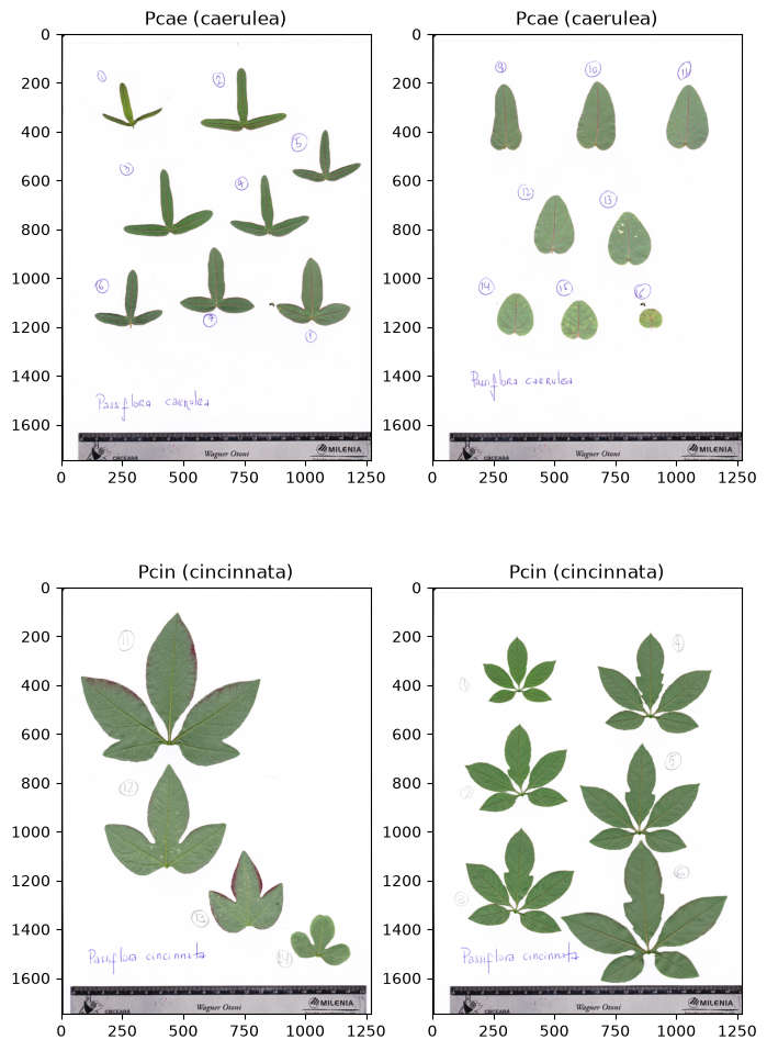
We use the Passiflora leaf scan dataset bundled with ktch: 25 flatbed scan images of 10 Passiflora species spanning simple elliptical to deeply lobed leaf forms. Each image contains multiple leaves from one plant individual, arranged from tip (youngest) to base (oldest). This dataset is a subset of the Passiflora leaf scan data from Chitwood & Otoni (2017) (data: Chitwood & Otoni, 2016).
data = load_image_passiflora_leaves(as_frame=True)

img_by_idx = {idx: img for idx, img in zip(data.meta.index, data.images)}
labels = {
    idx: f"{row.abbreviation} ({row.species})"
    for idx, row in data.meta.iterrows()
}

print(f"# of images: {len(data.images)}")
print(f"Species: {data.meta['species'].nunique()}")
print(data.meta[["abbreviation", "species"]].value_counts().sort_index())
Downloading data from 'https://pub-c1d6dba6c94843f88f0fd096d19c0831.r2.dev/datasets/image_passiflora_leaves/v2/image_passiflora_leaves.zip' to file '/home/runner/.cache/ktch-datasets/image_passiflora_leaves/v2/image_passiflora_leaves.zip'.
# of images: 25
Species: 10
abbreviation  species
Pcae          caerulea        2
Pcin          cincinnata      4
Pcor          coriacea        1
Pcri          cristalina      4
Pedu          edulis          5
Pgra          gracilis        3
Pmal          malacophylla    2
Pmis          misera          1
Prub          rubra           1
Psub          suberosa        2
Name: count, dtype: int64
fig, axes = plt.subplots(2, 2, figsize=(8, 12))
for ax, idx in zip(axes.flatten(), list(data.meta.index)[:4]):
    ax.imshow(img_by_idx[idx])
    ax.set_title(labels[idx])
We will digitize landmarks on individual leaves. Pick one scan to work with:
image_id = "Pcae1_1_8"
img = img_by_idx[image_id]

fig, ax = plt.subplots(figsize=(6, 8))
ax.imshow(img)
ax.set_title(labels[image_id])
Text(0.5, 1.0, 'Pcae (caerulea)')
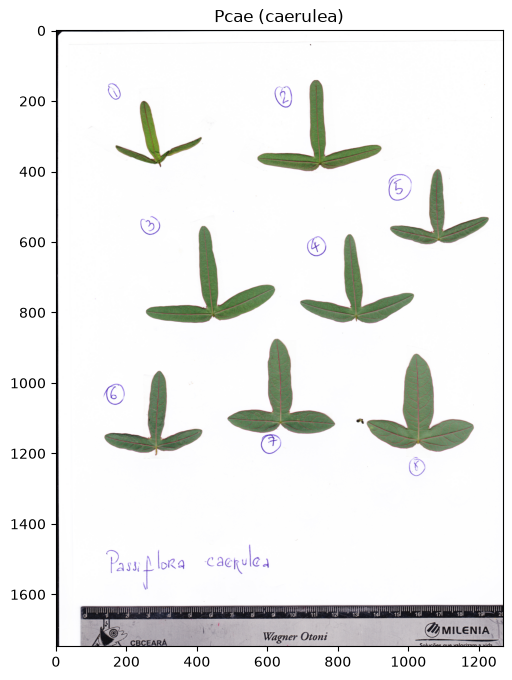
Image coordinate system#
In image coordinates, the origin is at the top-left corner. The x-axis points right and the y-axis points down. Landmark coordinates are recorded in this system.
Step 3: Digitize landmarks on a leaf#
Place landmarks interactively#
Each scan contains multiple leaves. Choose one leaf and place its 15 landmarks in order following the scheme described in Step 1. Left-click to add a point, right-click to undo the last point.
Note
This cell needs an interactive matplotlib backend, provided by
ipympl. Install it with pip install ipympl
in the same environment as your Jupyter kernel, restart the kernel, then run the
cell locally with %matplotlib widget in JupyterLab or VS Code. Capturing clicks
needs a live Python kernel, so the cell cannot run in the static documentation;
the two cells that follow render the view and the result instead, and the rest
of the tutorial uses pre-digitized landmarks so every output is reproducible.
If you get RuntimeError: 'widget' is not a recognised GUI loop or backend name,
ipympl is missing from the kernel’s environment or the kernel was not restarted
after installing it.
For digitizing large datasets, dedicated GUI tools are recommended; see Landmark-based Morphometrics for an overview.
%matplotlib widget

fig, ax = plt.subplots(figsize=(8, 8))
ax.imshow(img)
ax.set_title("Click to place landmarks (right-click to undo)")

landmarks = []
scatter = ax.scatter([], [], c="red", s=50, zorder=5)
texts = []


def on_click(event):
    if event.inaxes != ax:
        return
    if event.button == 1:  # left click: add
        landmarks.append([event.xdata, event.ydata])
    elif event.button == 3 and landmarks:  # right click: undo
        landmarks.pop()

    pts = np.array(landmarks) if landmarks else np.empty((0, 2))
    scatter.set_offsets(pts)

    for t in texts:
        t.remove()
    texts.clear()
    for i, (x, y) in enumerate(landmarks):
        texts.append(ax.annotate(str(i + 1), (x, y), fontsize=8,
                                 color="yellow", ha="center", va="bottom"))
    fig.canvas.draw_idle()


fig.canvas.mpl_connect("button_press_event", on_click)
landmarks
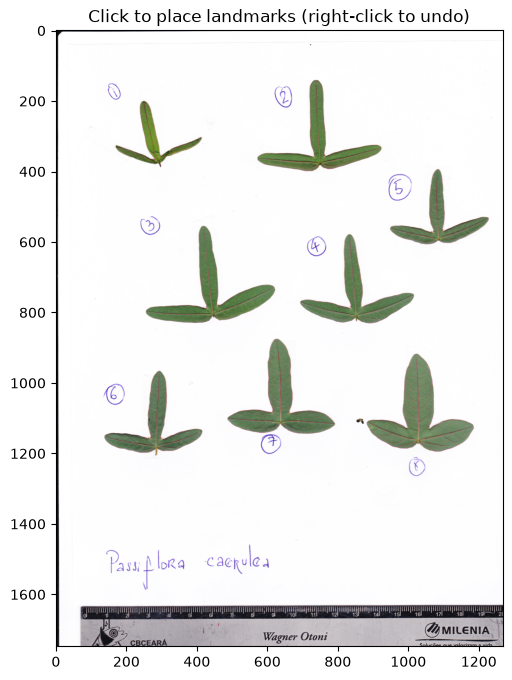
The digitization view#
The widget’s appearance is just an ordinary matplotlib figure; only the click handling needs a kernel. Rendered statically, the canvas you would interact with locally looks like this:
fig, ax = plt.subplots(figsize=(6, 8))
ax.imshow(img)
ax.set_title("Click to place landmarks (right-click to undo)")
Text(0.5, 1.0, 'Click to place landmarks (right-click to undo)')
Pre-digitized landmarks#
Because clicking needs a live kernel, the rest of this tutorial uses landmarks
digitized for 70 leaves of five species (P. caerulea,
P. cincinnata, P. coriacea, P. edulis, P. gracilis).
The coordinates are in the same image (pixel) coordinates the widget records,
so they drop straight into coords_list.
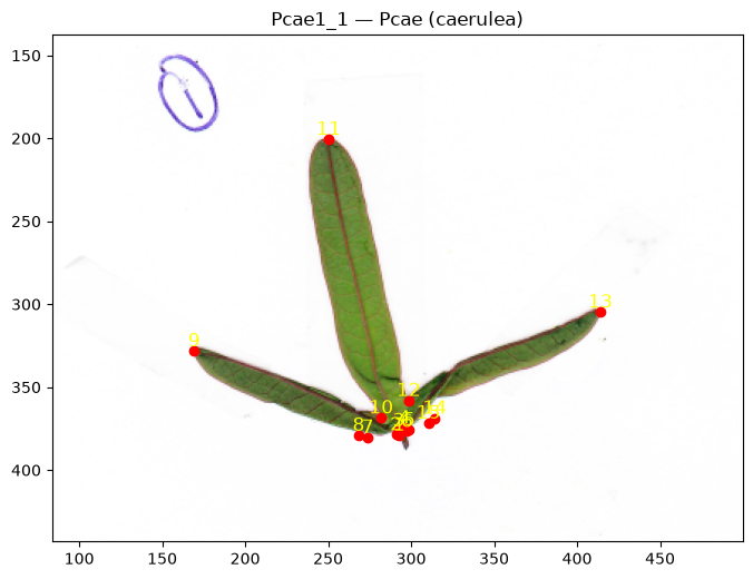
After placing the 15 landmarks#
This is what one digitized leaf looks like; the 15 landmarks of the first leaf of the chosen scan:
demo_idx = 0
demo_pts = coords_list[demo_idx]

fig, ax = plt.subplots(figsize=(8, 8))
ax.imshow(img)
ax.plot(demo_pts[:, 0], demo_pts[:, 1], "o", color="red", markersize=6)
for i, (x, y) in enumerate(demo_pts):
    ax.annotate(str(i + 1), (x, y), color="yellow", fontsize=12,
                ha="center", va="bottom")

# Zoom to the digitized leaf for legibility.
x0, y0 = demo_pts.min(0)
x1, y1 = demo_pts.max(0)
mx, my = 0.35 * (x1 - x0), 0.35 * (y1 - y0)
ax.set_xlim(x0 - mx, x1 + mx)
ax.set_ylim(y1 + my, y0 - my)
ax.set_title(f"{_LEAF_IDS[demo_idx]} — {labels[image_id]}")
Text(0.5, 1.0, 'Pcae1_1 — Pcae (caerulea)')
Step 4: Save the landmarks to TPS#
TPS is the standard landmark file format (see I/O and format conversion and Load TPS Files for the details).
write_tps stores the coordinates together with per-specimen metadata.
meta = pd.DataFrame(
    {"species": _SPECIES, "image_id": _IMAGE_IDS},
    index=pd.Index(_LEAF_IDS, name="leaf_id"),
)
meta.head()
| species | image_id | |
|---|---|---|
| leaf_id | ||
| Pcae1_1 | caerulea | Pcae1_1_8 |
| Pcae1_2 | caerulea | Pcae1_1_8 |
| Pcae1_3 | caerulea | Pcae1_1_8 |
| Pcae1_4 | caerulea | Pcae1_1_8 |
| Pcae1_5 | caerulea | Pcae1_1_8 |
tps_path = Path(tempfile.gettempdir()) / "passiflora_landmarks.tps"

write_tps(
    tps_path,
    coords_list,
    idx=meta.index.tolist(),
    image_path=[f"{idx}.png" for idx in meta["image_id"]],
    comments=meta["species"].tolist(),
)
Step 5: Aggregate into a multi-specimen dataset#
Reading the file back gives one record per specimen, from which we recover both the coordinates and the metadata we stored:
specimens = read_tps(tps_path)

coords_list = [t.to_numpy() for t in specimens]
leaf_ids = [t.specimen_name for t in specimens]
species = [t.comments for t in specimens]
image_ids = [Path(t.image_path).stem for t in specimens]

print(f"Specimens: {len(coords_list)}, landmarks each: {coords_list[0].shape[0]}")
pd.Series(species, name="count").value_counts().sort_index()
Specimens: 70, landmarks each: 15
count
caerulea      16
cincinnata    14
coriacea       7
edulis        15
gracilis      18
Name: count, dtype: int64
The coordinates can also be read directly as a tidy DataFrame with a
(specimen_id, coord_id) index:
read_tps(tps_path, as_frame=True).head()
| x | y | ||
|---|---|---|---|
| specimen_id | coord_id | ||
| Pcae1_1 | 0 | 292.8 | 378.8 |
| 1 | 291.0 | 378.6 | |
| 2 | 292.5 | 376.2 | |
| 3 | 296.0 | 374.6 | |
| 4 | 298.9 | 375.8 |
Verify landmarks on the source images#
Overlay one leaf per species on its scan to confirm the landmarks fall in the right place:
# Index of the first leaf of each species.
first_of_species = {}
for k, sp in enumerate(species):
    first_of_species.setdefault(sp, k)

fig, axes = plt.subplots(2, 3, figsize=(12, 9))
axes = axes.flatten()
for ax, (sp, k) in zip(axes, first_of_species.items()):
    plot_leaf(ax, img_by_idx[image_ids[k]], coords_list[k], title=f"{sp}\n{leaf_ids[k]}")

for ax in axes[len(first_of_species):]:
    ax.axis("off")
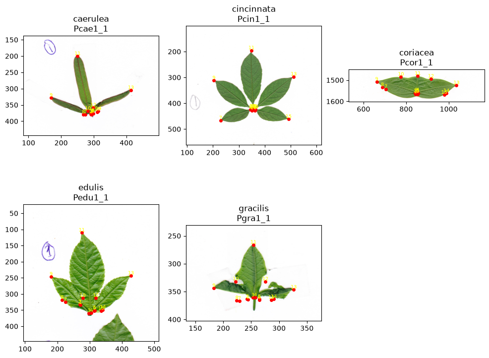
For P. gracilis, the first leaf was treated as deformed, and the landmarks were placed based on its assumed pre-deformation shape.
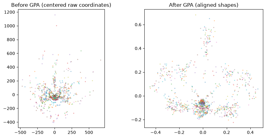
Step 6: Prepare for shape analysis#
Generalized Procrustes Analysis removes differences in position, scale, and
rotation, leaving only shape. It expects each specimen as a flat vector of
coordinates in (x, y) order, so we stack the landmark arrays into a 2-D array:
X = np.stack([lm.reshape(-1) for lm in coords_list])  # (n_specimens, n_landmarks * 2)

gpa = GeneralizedProcrustesAnalysis()
shapes = gpa.fit_transform(X)
fig, axes = plt.subplots(1, 2, figsize=(11, 5))

# Before GPA: raw configurations, centered for comparison.
for lm in coords_list:
    c = lm - lm.mean(0)
    axes[0].plot(c[:, 0], -c[:, 1], ".", alpha=0.3, markersize=3)
axes[0].set_aspect("equal")
axes[0].set_title("Before GPA (centered raw coordinates)")

# After GPA: Procrustes-aligned shapes.
for row in shapes:
    s = row.reshape(-1, 2)
    axes[1].plot(s[:, 0], -s[:, 1], ".", alpha=0.3, markersize=3)
axes[1].set_aspect("equal")
axes[1].set_title("After GPA (aligned shapes)")
Text(0.5, 1.0, 'After GPA (aligned shapes)')
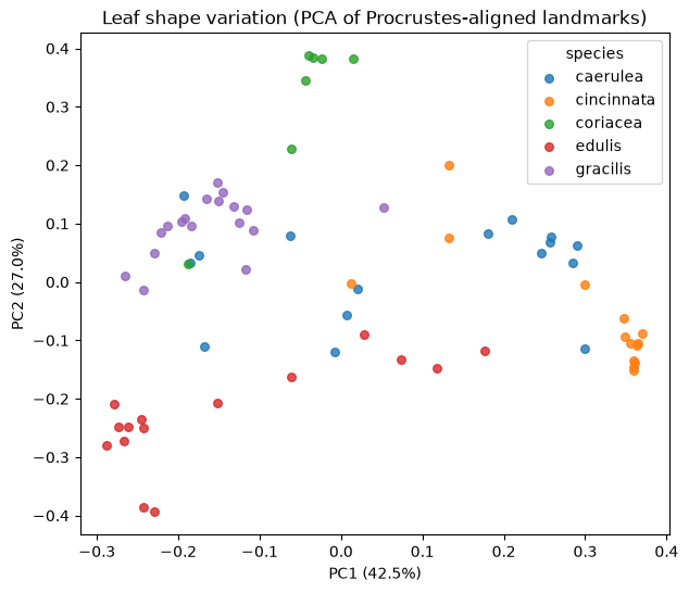
PCA of the aligned shapes shows how the five species are distributed in empirical morphospace:
pca = PCA(n_components=2)
scores = pca.fit_transform(shapes)
evr = pca.explained_variance_ratio_ * 100

species_arr = np.array(species)
fig, ax = plt.subplots(figsize=(7, 6))
for sp, color in zip(sorted(set(species)), plt.cm.tab10.colors):
    m = species_arr == sp
    ax.scatter(scores[m, 0], scores[m, 1], label=sp, color=color,
               s=30, alpha=0.8)
ax.set_xlabel(f"PC1 ({evr[0]:.1f}%)")
ax.set_ylabel(f"PC2 ({evr[1]:.1f}%)")
ax.legend(title="species")
ax.set_title("Leaf shape variation (PCA of Procrustes-aligned landmarks)")
Text(0.5, 1.0, 'Leaf shape variation (PCA of Procrustes-aligned landmarks)')
Summary#
This tutorial walked through a landmarking workflow: placing the 15 Passiflora landmarks on a scan, saving them to TPS together with their metadata, reading them back into a multi-specimen dataset, and running GPA followed by PCA. The digitized landmarks are ready for shape analysis with ktch.
Next steps#
Generalized Procrustes analysis - GPA with PCA in depth
Semilandmark analysis - combining landmarks with semilandmarks
Load TPS Files - reading and writing TPS files
Landmark-based Morphometrics - landmark theory and digitization approaches